MHKiT Wave Module

The following example runs an application of the MHKiT wave module to 1) read in NDBC data, 2) compute metrics from spectral data, 3) generate a capture length matrix, 4) calculate MAEP, and 5) plot the matrices.

Start by importing the necessary python packages and MHKiT module.

import numpy as np
import pandas as pd
from mhkit import wave

Load NDBC Data

We can use MHKiT to load data downloaded from https://www.ndbc.noaa.gov.

ndbc_data_file = 'data/wave/data.txt'

# ndbc.read_file outputs the NDBC file data into two variables.
    # raw_ndbc_data is a pandas DataFrame containing the file data.
    # meta contains the meta data, if available.
[raw_ndbc_data, meta] = wave.io.ndbc.read_file(ndbc_data_file)
raw_ndbc_data.head()

	0.0200	0.0325	0.0375	0.0425	0.0475	0.0525	0.0575	0.0625	0.0675	0.0725	...	0.3300	0.3400	0.3500	0.3650	0.3850	0.4050	0.4250	0.4450	0.4650	0.4850
2018-01-01 00:40:00	0.0	0.0	0.0	0.0	0.0	0.03	0.04	0.09	0.22	0.22	...	0.07	0.08	0.07	0.07	0.03	0.01	0.02	0.01	0.01	0.0
2018-01-01 01:40:00	0.0	0.0	0.0	0.0	0.0	0.02	0.06	0.08	0.21	0.21	...	0.07	0.07	0.08	0.02	0.01	0.02	0.01	0.01	0.00	0.0
2018-01-01 02:40:00	0.0	0.0	0.0	0.0	0.0	0.00	0.08	0.07	0.14	0.32	...	0.08	0.06	0.05	0.03	0.03	0.02	0.01	0.01	0.00	0.0
2018-01-01 03:40:00	0.0	0.0	0.0	0.0	0.0	0.00	0.13	0.22	0.26	0.32	...	0.05	0.06	0.05	0.03	0.03	0.01	0.01	0.00	0.00	0.0
2018-01-01 04:40:00	0.0	0.0	0.0	0.0	0.0	0.03	0.14	0.17	0.37	0.40	...	0.06	0.12	0.04	0.04	0.02	0.01	0.01	0.01	0.01	0.0

5 rows × 47 columns

The resulting DataFrame is spectra indexed (rows) by datetime with frequency as the columns. To use this data in MHKiT functions we must first transpose the DataFrame

# Transpose raw NDBC data
ndbc_data = raw_ndbc_data.T
ndbc_data.head()

	2018-01-01 00:40:00	2018-01-01 01:40:00	2018-01-01 02:40:00	2018-01-01 03:40:00	2018-01-01 04:40:00	2018-01-01 05:40:00	2018-01-01 06:40:00	2018-01-01 07:40:00	2018-01-01 08:40:00	2018-01-01 09:40:00	...	2018-01-31 14:40:00	2018-01-31 15:40:00	2018-01-31 16:40:00	2018-01-31 17:40:00	2018-01-31 18:40:00	2018-01-31 19:40:00	2018-01-31 20:40:00	2018-01-31 21:40:00	2018-01-31 22:40:00	2018-01-31 23:40:00
0.0200	0.0	0.0	0.0	0.0	0.0	0.00	0.0	0.0	0.0	0.0	...	0.00	0.0	0.0	0.0	0.00	0.0	0.0	0.0	0.0	0.0
0.0325	0.0	0.0	0.0	0.0	0.0	0.00	0.0	0.0	0.0	0.0	...	0.00	0.0	0.0	0.0	0.00	0.0	0.0	0.0	0.0	0.0
0.0375	0.0	0.0	0.0	0.0	0.0	0.00	0.0	0.0	0.0	0.0	...	0.00	0.0	0.0	0.0	0.00	0.0	0.0	0.0	0.0	0.0
0.0425	0.0	0.0	0.0	0.0	0.0	0.00	0.0	0.0	0.0	0.0	...	0.00	0.0	0.0	0.0	0.00	0.0	0.0	0.0	0.0	0.0
0.0475	0.0	0.0	0.0	0.0	0.0	0.01	0.0	0.0	0.0	0.0	...	0.06	0.0	0.0	0.0	0.07	0.0	0.0	0.0	0.0	0.0

5 rows × 743 columns

Compute Wave Metrics

We will now use MHKiT to compute the significant wave height, energy period, and energy flux.

# Compute the enegy periods from the NDBC spectra data
Te = wave.resource.energy_period(ndbc_data)
Te.head()

	Te
2018-01-01 00:40:00	7.458731
2018-01-01 01:40:00	7.682413
2018-01-01 02:40:00	7.498263
2018-01-01 03:40:00	7.676198
2018-01-01 04:40:00	7.669476

# Compute the significant wave height from the NDBC spectra data
Hm0 = wave.resource.significant_wave_height(ndbc_data)
Hm0.head()

	Hm0
2018-01-01 00:40:00	0.939574
2018-01-01 01:40:00	1.001399
2018-01-01 02:40:00	0.924770
2018-01-01 03:40:00	0.962497
2018-01-01 04:40:00	0.989949

# Set water depth to 60 m
h = 60

# Compute the energy flux  from the NDBC spectra data and water depth
J = wave.resource.energy_flux(ndbc_data,h)
J.head()

	J
2018-01-01 00:40:00	3354.825613
2018-01-01 01:40:00	3916.541523
2018-01-01 02:40:00	3278.298930
2018-01-01 03:40:00	3664.246679
2018-01-01 04:40:00	3867.014933

Conversion from DataFrames to Series

MHKiT functions typically take in Pandas Series so that the function knows exactly which column to use. Pandas Series are one-dimensional ndarrays with axis labels which are most commonly encountered when a single column is requested from a DataFrame (e.g. ndbc_data['2018-01-01 01:40:00'] returns a Pandas Series from the Pandas DataFrame of all frequencies at the specified time).

To the above results (energy Period, energy flux, and significant wave height) were returned as DataFrames. For DataFrames which only have one column the conversion from DataFrame to Series can accomplished using the squeeze method. Alternatively we can call on the column header. Both methods are demonstrated below:

# Convert the energy period DataFrame to a Series.
Te = Te.squeeze()
Te.head()

2018-01-01 00:40:00    7.458731
2018-01-01 01:40:00    7.682413
2018-01-01 02:40:00    7.498263
2018-01-01 03:40:00    7.676198
2018-01-01 04:40:00    7.669476
Name: Te, dtype: float64

# Alternatively, convert to Series by calling a specific column in the DataFrame
Hm0= Hm0['Hm0']
print(Hm0)

J  = J['J']
print(J)

2018-01-01 00:40:00    0.939574
2018-01-01 01:40:00    1.001399
2018-01-01 02:40:00    0.924770
2018-01-01 03:40:00    0.962497
2018-01-01 04:40:00    0.989949
                         ...
2018-01-31 19:40:00    2.650811
2018-01-31 20:40:00    3.086746
2018-01-31 21:40:00    2.650358
2018-01-31 22:40:00    2.941428
2018-01-31 23:40:00    2.895928
Name: Hm0, Length: 743, dtype: float64
2018-01-01 00:40:00     3354.825613
2018-01-01 01:40:00     3916.541523
2018-01-01 02:40:00     3278.298930
2018-01-01 03:40:00     3664.246679
2018-01-01 04:40:00     3867.014933
                           ...
2018-01-31 19:40:00    37596.750775
2018-01-31 20:40:00    52532.427635
2018-01-31 21:40:00    38153.227517
2018-01-31 22:40:00    50501.872907
2018-01-31 23:40:00    47070.874952
Name: J, Length: 743, dtype: float64

Generate Random Power Data

For demonstration purposes, this example uses synthetic power data generated from statistical distributions. In a real application, the user would provide power values from a WEC. The data is stored in pandas Series, containing 743 points.

# Set the random seed, to reproduce results
np.random.seed(1)
# Generate random power values
P = pd.Series(np.random.normal(200, 40, 743),index = J.index)

Capture Length Matrices

The following operations create capture length matrices, as specified by the IEC/TS 62600-100. But first, we need to calculate capture length and define bin centers. The mean capture length matrix is printed below. Keep in mind that this data has been artificially generated, so it may not be representative of what a real-world scatter diagram would look like.

# Calculate capture length
L = wave.performance.capture_length(P, J)

# Generate bins for Hm0 and Te, input format (start, stop, step_size)
Hm0_bins = np.arange(0, Hm0.values.max() + .5, .5)
Te_bins = np.arange(0, Te.values.max() + 1, 1)

# Create capture length matrices using mean, standard deviation, count, min and max statistics
LM_mean = wave.performance.capture_length_matrix(Hm0, Te, L, 'mean', Hm0_bins, Te_bins)
LM_std = wave.performance.capture_length_matrix(Hm0, Te, L, 'std', Hm0_bins, Te_bins)
LM_count = wave.performance.capture_length_matrix(Hm0, Te, L, 'count', Hm0_bins, Te_bins)
LM_min = wave.performance.capture_length_matrix(Hm0, Te, L, 'min', Hm0_bins, Te_bins)
LM_max = wave.performance.capture_length_matrix(Hm0, Te, L, 'max', Hm0_bins, Te_bins)

# Show mean capture length matrix
LM_mean

	0.0	1.0	2.0	3.0	4.0	5.0	6.0	7.0	8.0	9.0	10.0	11.0	12.0	13.0	14.0	15.0	16.0
0.0	NaN	NaN	NaN	NaN	NaN	NaN	NaN	NaN	NaN	NaN	NaN	NaN	NaN	NaN	NaN	NaN	NaN
0.5	NaN	NaN	NaN	NaN	NaN	NaN	NaN	0.120286	0.053376	NaN	NaN	NaN	NaN	NaN	NaN	NaN	NaN
1.0	NaN	NaN	NaN	NaN	NaN	NaN	0.110686	0.068070	0.049452	0.065912	NaN	0.056593	0.029950	0.017234	NaN	NaN	NaN
1.5	NaN	NaN	NaN	NaN	NaN	NaN	NaN	0.019749	0.018673	NaN	NaN	0.012473	0.011205	0.012307	0.010432	NaN	NaN
2.0	NaN	NaN	NaN	NaN	NaN	NaN	NaN	0.013882	0.012547	0.009672	0.008770	0.008585	0.007525	0.005272	0.007809	NaN	NaN
2.5	NaN	NaN	NaN	NaN	NaN	NaN	NaN	NaN	0.007244	0.006488	0.005788	0.005652	0.005180	0.004260	0.003623	0.004509	NaN
3.0	NaN	NaN	NaN	NaN	NaN	NaN	NaN	0.004500	0.005660	0.004691	0.004109	0.003952	0.003104	0.003408	0.002291	0.001792	NaN
3.5	NaN	NaN	NaN	NaN	NaN	NaN	NaN	NaN	0.003924	0.003674	0.003020	0.002746	0.002247	0.002000	0.002257	0.002033	NaN
4.0	NaN	NaN	NaN	NaN	NaN	NaN	NaN	NaN	0.003185	0.002513	0.002386	0.002147	0.002246	0.001605	0.001730	NaN	NaN
4.5	NaN	NaN	NaN	NaN	NaN	NaN	NaN	NaN	0.002343	0.002087	0.001919	0.001590	0.001438	NaN	NaN	NaN	NaN
5.0	NaN	NaN	NaN	NaN	NaN	NaN	NaN	NaN	0.001913	0.001720	0.001716	0.001411	0.001219	0.001345	NaN	NaN	NaN
5.5	NaN	NaN	NaN	NaN	NaN	NaN	NaN	NaN	0.002101	0.001516	0.001331	0.000902	0.001033	NaN	NaN	NaN	NaN
6.0	NaN	NaN	NaN	NaN	NaN	NaN	NaN	NaN	NaN	0.001097	0.000895	NaN	0.000858	0.000987	NaN	NaN	NaN
6.5	NaN	NaN	NaN	NaN	NaN	NaN	NaN	NaN	NaN	0.000837	0.001024	0.000419	NaN	0.000688	NaN	NaN	NaN
7.0	NaN	NaN	NaN	NaN	NaN	NaN	NaN	NaN	NaN	NaN	NaN	NaN	0.000461	0.000633	NaN	NaN	NaN
7.5	NaN	NaN	NaN	NaN	NaN	NaN	NaN	NaN	NaN	NaN	0.000553	NaN	NaN	0.000312	0.000437	NaN	NaN
8.0	NaN	NaN	NaN	NaN	NaN	NaN	NaN	NaN	NaN	NaN	NaN	NaN	NaN	NaN	0.000443	0.000351	NaN
8.5	NaN	NaN	NaN	NaN	NaN	NaN	NaN	NaN	NaN	NaN	NaN	NaN	NaN	NaN	NaN	0.000418	0.000405
9.0	NaN	NaN	NaN	NaN	NaN	NaN	NaN	NaN	NaN	NaN	NaN	NaN	NaN	NaN	NaN	NaN	NaN
9.5	NaN	NaN	NaN	NaN	NaN	NaN	NaN	NaN	NaN	NaN	NaN	NaN	NaN	NaN	NaN	0.000153	NaN
10.0	NaN	NaN	NaN	NaN	NaN	NaN	NaN	NaN	NaN	NaN	NaN	NaN	NaN	NaN	NaN	NaN	0.000281
10.5	NaN	NaN	NaN	NaN	NaN	NaN	NaN	NaN	NaN	NaN	NaN	NaN	NaN	NaN	NaN	0.000204	0.000225

Additional capture length matrices can be computed, for example, the frequency matrix is computed below.

# Create capture length matrices using frequency
LM_freq = wave.performance.capture_length_matrix(Hm0, Te, L,'frequency', Hm0_bins, Te_bins)

# Show capture length matrix using frequency
LM_freq

	0.0	1.0	2.0	3.0	4.0	5.0	6.0	7.0	8.0	9.0	10.0	11.0	12.0	13.0	14.0	15.0	16.0
0.0	0.0	0.0	0.0	0.0	0.0	0.0	0.000000	0.000000	0.000000	0.000000	0.000000	0.000000	0.000000	0.000000	0.000000	0.000000	0.000000
0.5	0.0	0.0	0.0	0.0	0.0	0.0	0.000000	0.002692	0.001346	0.000000	0.000000	0.000000	0.000000	0.000000	0.000000	0.000000	0.000000
1.0	0.0	0.0	0.0	0.0	0.0	0.0	0.001346	0.006729	0.004038	0.001346	0.000000	0.002692	0.002692	0.001346	0.000000	0.000000	0.000000
1.5	0.0	0.0	0.0	0.0	0.0	0.0	0.000000	0.005384	0.002692	0.000000	0.000000	0.009421	0.004038	0.006729	0.005384	0.000000	0.000000
2.0	0.0	0.0	0.0	0.0	0.0	0.0	0.000000	0.002692	0.005384	0.018843	0.018843	0.029610	0.021534	0.001346	0.002692	0.000000	0.000000
2.5	0.0	0.0	0.0	0.0	0.0	0.0	0.000000	0.000000	0.013459	0.052490	0.055182	0.018843	0.025572	0.022880	0.005384	0.001346	0.000000
3.0	0.0	0.0	0.0	0.0	0.0	0.0	0.000000	0.001346	0.021534	0.044415	0.047106	0.020188	0.012113	0.010767	0.010767	0.001346	0.000000
3.5	0.0	0.0	0.0	0.0	0.0	0.0	0.000000	0.000000	0.006729	0.040377	0.029610	0.047106	0.004038	0.008075	0.004038	0.001346	0.000000
4.0	0.0	0.0	0.0	0.0	0.0	0.0	0.000000	0.000000	0.009421	0.017497	0.029610	0.040377	0.002692	0.004038	0.005384	0.000000	0.000000
4.5	0.0	0.0	0.0	0.0	0.0	0.0	0.000000	0.000000	0.016151	0.013459	0.017497	0.022880	0.012113	0.000000	0.000000	0.000000	0.000000
5.0	0.0	0.0	0.0	0.0	0.0	0.0	0.000000	0.000000	0.002692	0.008075	0.008075	0.010767	0.022880	0.001346	0.000000	0.000000	0.000000
5.5	0.0	0.0	0.0	0.0	0.0	0.0	0.000000	0.000000	0.001346	0.012113	0.006729	0.004038	0.014805	0.000000	0.000000	0.000000	0.000000
6.0	0.0	0.0	0.0	0.0	0.0	0.0	0.000000	0.000000	0.000000	0.002692	0.002692	0.000000	0.005384	0.001346	0.000000	0.000000	0.000000
6.5	0.0	0.0	0.0	0.0	0.0	0.0	0.000000	0.000000	0.000000	0.002692	0.002692	0.001346	0.000000	0.002692	0.000000	0.000000	0.000000
7.0	0.0	0.0	0.0	0.0	0.0	0.0	0.000000	0.000000	0.000000	0.000000	0.000000	0.000000	0.001346	0.004038	0.000000	0.000000	0.000000
7.5	0.0	0.0	0.0	0.0	0.0	0.0	0.000000	0.000000	0.000000	0.000000	0.001346	0.000000	0.000000	0.001346	0.008075	0.000000	0.000000
8.0	0.0	0.0	0.0	0.0	0.0	0.0	0.000000	0.000000	0.000000	0.000000	0.000000	0.000000	0.000000	0.000000	0.002692	0.002692	0.000000
8.5	0.0	0.0	0.0	0.0	0.0	0.0	0.000000	0.000000	0.000000	0.000000	0.000000	0.000000	0.000000	0.000000	0.000000	0.001346	0.001346
9.0	0.0	0.0	0.0	0.0	0.0	0.0	0.000000	0.000000	0.000000	0.000000	0.000000	0.000000	0.000000	0.000000	0.000000	0.000000	0.000000
9.5	0.0	0.0	0.0	0.0	0.0	0.0	0.000000	0.000000	0.000000	0.000000	0.000000	0.000000	0.000000	0.000000	0.000000	0.001346	0.000000
10.0	0.0	0.0	0.0	0.0	0.0	0.0	0.000000	0.000000	0.000000	0.000000	0.000000	0.000000	0.000000	0.000000	0.000000	0.000000	0.001346
10.5	0.0	0.0	0.0	0.0	0.0	0.0	0.000000	0.000000	0.000000	0.000000	0.000000	0.000000	0.000000	0.000000	0.000000	0.001346	0.001346

The capture_length_matrix function can also be used as an arbitrary matrix generator. To do this, simply pass a different Series in the place of capture length (L). For example, while not specified by the IEC standards, if the user doesn’t have the omnidirectional wave flux, the average power matrix could hypothetically be generated in the following manner.

# Demonstration of arbitrary matrix generator
PM_mean_not_standard = wave.performance.capture_length_matrix(Hm0, Te, P, 'mean', Hm0_bins, Te_bins)

The capture_length_matrix function can also use a callable function as the statistic argument. For example, suppose that we wanted to generate a matrix with the variance of the capture length. We could achieve this by passing the NumPy variance function np.var into the capture_length_matrix function, as shown below.

# Demonstration of passing a callable function to the matrix generator
LM_variance = wave.performance.capture_length_matrix(Hm0, Te, L, np.var, Hm0_bins, Te_bins)

Power Matrices

As specified in IEC/TS 62600-100, the power matrix is generated from the capture length matrix and wave energy flux matrix, as shown below

# Create wave energy flux matrix using mean
JM = wave.performance.wave_energy_flux_matrix(Hm0, Te, J, 'mean', Hm0_bins, Te_bins)

# Create power matrix using mean
PM_mean = wave.performance.power_matrix(LM_mean, JM)

# Create power matrix using standard deviation
PM_std = wave.performance.power_matrix(LM_std, JM)

# Show mean power matrix, round to 3 decimals
PM_mean.round(3)

	0.0	1.0	2.0	3.0	4.0	5.0	6.0	7.0	8.0	9.0	10.0	11.0	12.0	13.0	14.0	15.0	16.0
0.0	NaN	NaN	NaN	NaN	NaN	NaN	NaN	NaN	NaN	NaN	NaN	NaN	NaN	NaN	NaN	NaN	NaN
0.5	NaN	NaN	NaN	NaN	NaN	NaN	NaN	224.996	117.594	NaN	NaN	NaN	NaN	NaN	NaN	NaN	NaN
1.0	NaN	NaN	NaN	NaN	NaN	NaN	212.762	202.713	188.707	187.103	NaN	213.926	174.154	164.886	NaN	NaN	NaN
1.5	NaN	NaN	NaN	NaN	NaN	NaN	NaN	176.402	199.802	NaN	NaN	201.883	191.598	221.705	190.124	NaN	NaN
2.0	NaN	NaN	NaN	NaN	NaN	NaN	NaN	203.667	216.857	192.965	201.633	216.268	209.634	162.569	232.530	NaN	NaN
2.5	NaN	NaN	NaN	NaN	NaN	NaN	NaN	NaN	193.397	203.529	196.907	212.883	211.277	202.760	199.263	272.421	NaN
3.0	NaN	NaN	NaN	NaN	NaN	NaN	NaN	170.739	216.459	197.484	200.895	212.107	193.837	222.185	169.497	122.296	NaN
3.5	NaN	NaN	NaN	NaN	NaN	NaN	NaN	NaN	194.894	214.108	202.725	206.901	184.099	186.077	221.659	186.201	NaN
4.0	NaN	NaN	NaN	NaN	NaN	NaN	NaN	NaN	217.289	189.403	201.362	207.532	207.971	172.771	213.854	NaN	NaN
4.5	NaN	NaN	NaN	NaN	NaN	NaN	NaN	NaN	197.994	194.238	205.559	203.195	197.980	NaN	NaN	NaN	NaN
5.0	NaN	NaN	NaN	NaN	NaN	NaN	NaN	NaN	198.149	196.527	222.219	215.221	204.002	254.004	NaN	NaN	NaN
5.5	NaN	NaN	NaN	NaN	NaN	NaN	NaN	NaN	249.158	212.561	212.734	168.655	208.220	NaN	NaN	NaN	NaN
6.0	NaN	NaN	NaN	NaN	NaN	NaN	NaN	NaN	NaN	182.314	159.418	NaN	208.418	241.347	NaN	NaN	NaN
6.5	NaN	NaN	NaN	NaN	NaN	NaN	NaN	NaN	NaN	164.712	233.890	110.517	NaN	207.919	NaN	NaN	NaN
7.0	NaN	NaN	NaN	NaN	NaN	NaN	NaN	NaN	NaN	NaN	NaN	NaN	155.691	229.022	NaN	NaN	NaN
7.5	NaN	NaN	NaN	NaN	NaN	NaN	NaN	NaN	NaN	NaN	166.855	NaN	NaN	128.897	198.053	NaN	NaN
8.0	NaN	NaN	NaN	NaN	NaN	NaN	NaN	NaN	NaN	NaN	NaN	NaN	NaN	NaN	230.281	184.510	NaN
8.5	NaN	NaN	NaN	NaN	NaN	NaN	NaN	NaN	NaN	NaN	NaN	NaN	NaN	NaN	NaN	248.338	264.534
9.0	NaN	NaN	NaN	NaN	NaN	NaN	NaN	NaN	NaN	NaN	NaN	NaN	NaN	NaN	NaN	NaN	NaN
9.5	NaN	NaN	NaN	NaN	NaN	NaN	NaN	NaN	NaN	NaN	NaN	NaN	NaN	NaN	NaN	116.230	NaN
10.0	NaN	NaN	NaN	NaN	NaN	NaN	NaN	NaN	NaN	NaN	NaN	NaN	NaN	NaN	NaN	NaN	244.634
10.5	NaN	NaN	NaN	NaN	NaN	NaN	NaN	NaN	NaN	NaN	NaN	NaN	NaN	NaN	NaN	190.849	212.411

Calculate MAEP

There are two ways to calculate the mean annual energy production (MEAP). One is from capture length and wave energy flux matrices, the other is from time-series data, as shown below.

# Calcaulte maep from timeseries
maep_timeseries = wave.performance.mean_annual_energy_production_timeseries(L, J)
print("MAEP from timeseries = ", maep_timeseries)

# Calcaulte maep from matrix
maep_matrix = wave.performance.mean_annual_energy_production_matrix(LM_mean, JM, LM_freq)
print("MAEP from matrices = ", maep_matrix)

MAEP from timeseries =  1767087.527586333
MAEP from matrices =  1781210.8652839188

Graphics

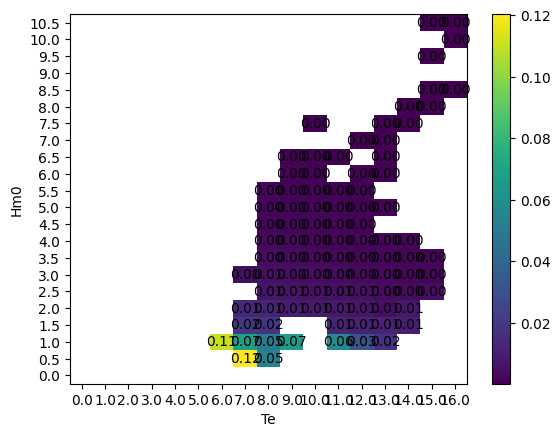
The graphics function plot_matrix can be used to visualize results. It is important to note that the plotting function assumes the step size between bins to be linear.

# Plot the capture length mean matrix
ax = wave.graphics.plot_matrix(LM_mean)

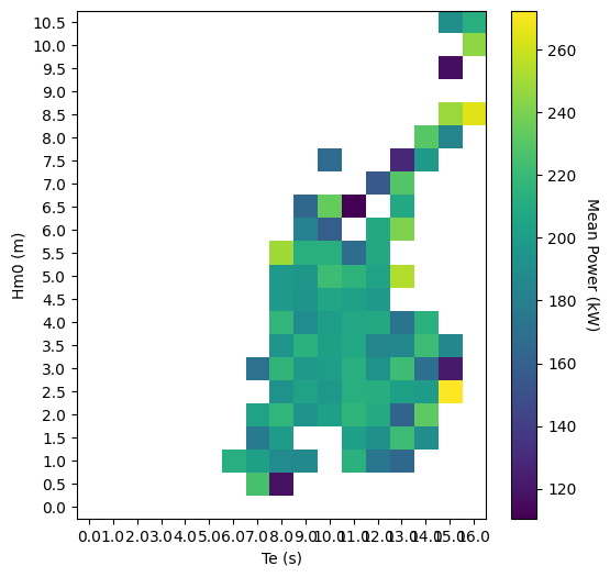
The plotting function only requires the matrix as input, but the function can also take several other arguments. The list of optional arguments is: xlabel, ylabel, zlabel, show_values, and ax. The following uses these optional arguments. The matplotlib package is imported to define an axis with a larger figure size.

# Customize the matrix plot
import matplotlib.pylab as plt
plt.figure(figsize=(6,6))
ax = plt.gca()
wave.graphics.plot_matrix(PM_mean, xlabel='Te (s)', ylabel='Hm0 (m)', \
              zlabel='Mean Power (kW)', show_values=False, ax=ax)

<AxesSubplot:xlabel='Te (s)', ylabel='Hm0 (m)'>