Delft3D IO Module
The following example will familiarize the user with using the Delft3D (d3d) toolbox in MHKiT-Python. d3d can be used to plot the data from a NetCDF output from Delft3D SNL-D3D-CEC-FM. The example will walk through a flume case with a turbine. The flume is 18 m long, 4 m wide and 2m deep with the turbine placed at 6 m along the length and 3 m along the width. The turbine used for this simulation has a circular cross-section with a diameter
of 0.7m, a thrust coefficient of 0.72, and a power coefficient of 0.45. The simulation was run with 5 depth layers and 5-time intervals over 4 min.
This example will show how to create a centerline plot at a desired depth for different variables outputs of Delft3D using matplotlib. It will also show how to make a contour plot of a given plane or depth for the variable output by Delft3D and how to use those variables to calculate turbulence intensity. This module can be helpful to visualize the wake of a turbine and help predict how a turbine will affect the surrounding area.
Start by importing the necessary python packages and MHKiT module.
[1]:
from os.path import abspath, dirname, join, normpath, relpath
from mhkit.river.io import d3d
from math import isclose
import scipy.interpolate as interp
import matplotlib.pyplot as plt
import numpy as np
import pandas as pd
import netCDF4

plt.rcParams.update({"font.size": 15})  # Set font size of plots title and labels
Loading Data from Delft3D as a NetCDF
A NetCDF file has been saved in the \MHKiT-Python\examples\data\river\d3d directory of a simple flume case with a turbine for reference data. Here we are inputting strings for the file path datadir, and file name filename, so the NetCDF file can be saved as a NetCDF object using the python pack netCDF4 under the variable d3d_data.
There are many variables saved in the NetCDF object d3d_data. The function d3d_data.variables.keys() returns a dictionary of the available data. Here we look at the dictionary keys output to see all the variables.
[2]:
# Downloading Data
datadir = normpath(join(relpath(join("data", "river", "d3d"))))
filename = "turbineTest_map.nc"
d3d_data = netCDF4.Dataset(join(datadir, filename))

# Printing variable and description
for var in d3d_data.variables.keys():
    try:
        d3d_data[var].long_name
    except:
        print(f'"{var}"')
    else:
        print(f'"{var}": {d3d_data[var].long_name}')
"mesh2d_enc_x": x-coordinate
"mesh2d_enc_y": y-coordinate
"mesh2d_enc_node_count": count of coordinates in each instance geometry
"mesh2d_enc_part_node_count": count of nodes in each geometry part
"mesh2d_enc_interior_ring": type of each geometry part
"mesh2d_enclosure_container"
"Mesh2D"
"NetNode_x": x-coordinate
"NetNode_y": y-coordinate
"projected_coordinate_system"
"NetNode_z": bed level at net nodes (flow element corners)
"NetLink": link between two netnodes
"NetLinkType": type of netlink
"NetElemNode": mapping from net cell to net nodes (counterclockwise)
"NetElemLink": mapping from net cell to its net links (counterclockwise)
"NetLinkContour_x": list of x-contour points of momentum control volume surrounding each net/flow link
"NetLinkContour_y": list of y-contour points of momentum control volume surrounding each net/flow link
"NetLink_xu": x-coordinate of net link center (velocity point)
"NetLink_yu": y-coordinate of net link center (velocity point)
"BndLink": netlinks that compose the net boundary
"FlowElem_xcc": x-coordinate of flow element circumcenter
"FlowElem_ycc": y-coordinate of flow element circumcenter
"FlowElem_zcc": bed level of flow element
"FlowElem_bac": flow element area
"FlowElem_xzw": x-coordinate of flow element center of mass
"FlowElem_yzw": y-coordinate of flow element center of mass
"FlowElemContour_x": list of x-coordinates forming flow element
"FlowElemContour_y": list of y-coordinates forming flow element
"FlowElem_bl": Initial bed level at flow element circumcenter
"ElemLink": flow nodes between/next to which link between two netnodes lies
"FlowLink": link/interface between two flow elements
"FlowLinkType": type of flowlink
"FlowLink_xu": x-coordinate of flow link center (velocity point)
"FlowLink_yu": y-coordinate of flow link center (velocity point)
"FlowLink_lonu": longitude
"FlowLink_latu": latitude
"time"
"LayCoord_cc": sigma layer coordinate at flow element center
"LayCoord_w": sigma layer coordinate at vertical interface
"timestep"
"s1": water level
"waterdepth": water depth
"unorm": normal component of sea_water_speed
"ucz": upward velocity on flow element center
"ucxa": depth-averaged velocity on flow element center, x-component
"ucya": depth-averaged velocity on flow element center, y-component
"ww1": upward velocity on vertical interface
"ucx": velocity on flow element center, x-component
"ucy": velocity on flow element center, y-component
"turkin1": turbulent kinetic energy
"vicwwu": turbulent vertical eddy viscosity
"tureps1": turbulent energy dissipation
Seconds Run and Time Index
The 'time_index' can be used to pull data from different instances in time. For the example data included there are 5-time steps meaning we have indexes in the range 0 and to 4. Each time index has an associated 'seconds_run' that quantifies the number of seconds that passed from the start of the simulation. To get all of the 'seconds_run' for a data set use the function get_all_time the output is an array of all the 'seconds_run' for the input data set.
[3]:
time = d3d.get_all_time(d3d_data)
print(time)
[ 0. 60. 120. 180. 240.]
To convert from a 'seconds_run' to a 'time_index' or vice versa. The inputs are a netcdf data set, then a 'time_index'. This example shows what happens if you input a 'seconds_run' that is close to but not exactly a 'seconds_run' associated with a 'time_idex'. The function will throw a warning and return the closest time index.
[4]:
seconds_run = 62
time_index = d3d._convert_time(d3d_data, seconds_run=seconds_run)
print(time_index)
1
C:\Users\sterl\AppData\Local\Temp\ipykernel_21668\3610353735.py:2: UserWarning: Warning: seconds_run not found. Closest time stampfound 60.0
  time_index = d3d._convert_time(d3d_data, seconds_run=seconds_run)
Dataframe from NetCDF
For this example we will create a DataFrame from the D3d NetCDF object using the variable 'ucx', the velocity in the x-direction (see available data in previous block output). MHKiT’s d3d function get_all_data_points will pull all the raw data from the NetCDF file for the specified variable at a specific time index in a dataframe var_data_df. The time_index can be used to pull data from a different instances in time (the last valid time_index, time_index=-1, is the
default setting). If an integer outside of the valid range is entered the code will output an error with the max valid output listed. The output data from get_all_data_points will be the position (x, y, waterdepth) in meters, the value of vairable in meters per second and the run time of the simulation in seconds or 'x', 'y', 'waterdepth', 'waterlevel', ‘ucx’, and 'time'. The time run in simulation varies based on the ‘time_step’.
The limits max_plot_vel and min_plot_vel are defined to bound the plots of the variable’s data in the next 3 example plots.
[5]:
# Getting variable data
variable = "ucx"
var_data_df = d3d.get_all_data_points(d3d_data, variable, time_index=4)
print(var_data_df)

# Setting plot limits
max_plot_vel = 1.25
min_plot_vel = 0.5
            x      y  waterdepth  waterlevel       ucx   time
index
0       0.125  1.125    0.199485   -0.005154  0.717881  240.0
1       0.375  1.125    0.200008    0.000081  0.689645  240.0
2       0.125  1.375    0.199485   -0.005154  0.717881  240.0
3       0.625  1.125    0.200056    0.000559  0.694164  240.0
4       0.375  1.375    0.200008    0.000081  0.689645  240.0
...       ...    ...         ...         ...       ...    ...
5755   17.625  4.625    1.794649   -0.005946  1.245117  240.0
5756   17.375  4.875    1.794848   -0.005724  1.222989  240.0
5757   17.875  4.625    1.799824   -0.000196  1.255866  240.0
5758   17.625  4.875    1.794638   -0.005958  1.245292  240.0
5759   17.875  4.875    1.799828   -0.000191  1.256067  240.0

[5760 rows x 6 columns]
Plotting a Line Plot Between Two Points
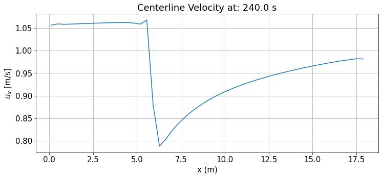
To view the maximum wake effect of the turbine we can plot a velocity down the centerline of the flume. To do this we will create an array between two points down the center of the flume. We will then interpolate the grided data results onto our centerline array. Since the flume is retangular the centerline points are found by taking the average of the maximum and minimum value for the width, y, and the waterdepth, of the flume. We will then input one array, x, and two points, y
and waterdepth into the function create_points to create our centerline array to interpolate over. The function create_points will then output a dataframe, cline_points, with keys 'x', 'y', and 'waterdepth'.
[6]:
# Use rectangular grid min and max to find flume centerline
xmin = var_data_df.x.max()
xmax = var_data_df.x.min()

ymin = var_data_df.y.max()
ymax = var_data_df.y.min()

waterdepth_min = var_data_df.waterdepth.max()
waterdepth_max = var_data_df.waterdepth.min()

# Creating one array and 2 points
x = np.linspace(xmin, xmax)
y = np.mean([ymin, ymax])
waterdepth = np.mean([waterdepth_min, waterdepth_max])

# Creating an array of points
cline_points = d3d.create_points(x, y, waterdepth)
cline_points.head()
[6]:
| x | y | waterdepth | |
|---|---|---|---|
| index | |||
| 0 | 17.875000 | 3.0 | 1.000931 |
| 1 | 17.512755 | 3.0 | 1.000931 |
| 2 | 17.150510 | 3.0 | 1.000931 |
| 3 | 16.788265 | 3.0 | 1.000931 |
| 4 | 16.426020 | 3.0 | 1.000931 |
Next the variable ucx is interpolated onto the created cline_points using scipy interp function and saved as cline_variable. The results are then plotted for velocity in the x direction, ucx, along the length of the flume, x.
[7]:
# Interpolate raw data onto the centerline
cline_variable = interp.griddata(
    var_data_df[["x", "y", "waterdepth"]],
    var_data_df[variable],
    cline_points[["x", "y", "waterdepth"]],
)

# Plotting
plt.figure(figsize=(12, 5))
plt.plot(x, cline_variable)

plt.grid()
plt.xlabel("x (m)")
plt.ylabel("$u_x$ [m/s]")
plt.title(f"Centerline Velocity at: {var_data_df.time[1]} s")
[7]:
Text(0.5, 1.0, 'Centerline Velocity at: 240.0 s')
Contour Plot for a Given Sigma Layer
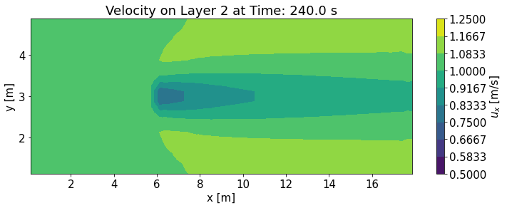
Sometimes it is useful to plot only the raw data of a given layer. Using get_layer_data a single layer of raw data will be retrieved from the NetCDF object. The d3d function ,get_layer_data takes 3 inputs, the NetCDF object (d3d_data), a variable name as a string (variable), and the layer to retrieve (layer) as an integer. The variable is set to the velocity in the x direction, 'ucx', and the layer of data to plot as 2. Since there are 5 sigma layers in this example
layer 2 is approximately the middle layer. layer works as an index that begins at begins at 0 and ends at 4. The get_layer_data then outputs a dataframe layer_data with the keys 'x', 'y', 'waterdepth', 'waterlevel', 'v', and 'time' as the length, width, waterdepth, value, and run time of simulation of the specified variable in this case velocity in the x direction, ‘ucx’.
To plot the data the maximum and minimum, max_plot_vel and min_plot_vel, values are pulled from above to limit bounds of the color bar to show the value of the specified variable, in this case it’s velocity in the x direction. The type of plot is also defined as a string ‘contour’ to add to the title of the plot.
[8]:
# Get layer data
layer = 2
layer_data = d3d.get_layer_data(d3d_data, variable, layer)

# Plotting
plt.figure(figsize=(12, 4))
contour_plot = plt.tricontourf(
    layer_data.x,
    layer_data.y,
    layer_data.v,
    vmin=min_plot_vel,
    vmax=max_plot_vel,
    levels=np.linspace(min_plot_vel, max_plot_vel, 10),
)

cbar = plt.colorbar(contour_plot)
cbar.set_label("$u_x$ [m/s]")

plt.xlabel("x [m]")
plt.ylabel("y [m]")
plt.title(f"Velocity on Layer {layer} at Time: {layer_data.time[1]} s")
[8]:
Text(0.5, 1.0, 'Velocity on Layer 2 at Time: 240.0 s')
Plotting a Contour Plot of a given Plane
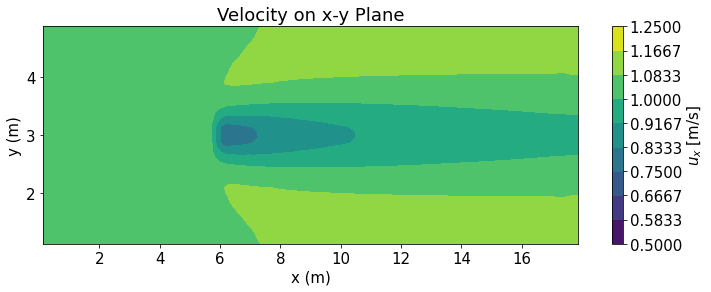
If you wanted to look at a contour plot of a specific waterdepth you can create a contour plot over given points. Expanding on the centerline array points we can create a grid using the same create_points function by inputting two arrays along the length of the flume, x , and width of the flume, y_contour , and one point for the waterdepth we want to look at. create_points then outputs a dataframe contour_points of points to calculate the contour values over with the keys
'x', 'y', and 'waterdepth'.
[9]:
# Create x-y plane at z level midpoint
x2 = np.linspace(xmin, xmax, num=100)
y_contour = np.linspace(ymin, ymax, num=40)
z2 = np.mean([waterdepth_min, waterdepth_max])

contour_points = d3d.create_points(x2, y_contour, z2)
contour_points
[9]:
| x | y | waterdepth | |
|---|---|---|---|
| index | |||
| 0 | 17.875000 | 4.875 | 1.000931 |
| 1 | 17.695707 | 4.875 | 1.000931 |
| 2 | 17.516414 | 4.875 | 1.000931 |
| 3 | 17.337121 | 4.875 | 1.000931 |
| 4 | 17.157828 | 4.875 | 1.000931 |
| ... | ... | ... | ... |
| 3995 | 0.842172 | 1.125 | 1.000931 |
| 3996 | 0.662879 | 1.125 | 1.000931 |
| 3997 | 0.483586 | 1.125 | 1.000931 |
| 3998 | 0.304293 | 1.125 | 1.000931 |
| 3999 | 0.125000 | 1.125 | 1.000931 |
4000 rows × 3 columns
Next the data is interpolated on to the points created and saved as an arrray under the variable name contour_variable.
[10]:
contour_variable = interp.griddata(
    var_data_df[["x", "y", "waterdepth"]],
    var_data_df[variable],
    contour_points[["x", "y", "waterdepth"]],
)
The results are then plotted. The minimum and maximum values show on the graph are pulled from above (max_plot_vel and min_plot_vel) as in the previous example. The contour plot of the velocity is then output at the center waterdepth of the flume.
[11]:
# Plotting
plt.figure(figsize=(12, 4))
contour_plot = plt.tricontourf(
    contour_points.x,
    contour_points.y,
    contour_variable,
    vmin=min_plot_vel,
    vmax=max_plot_vel,
    levels=np.linspace(min_plot_vel, max_plot_vel, 10),
)

plt.xlabel("x (m)")
plt.ylabel("y (m)")
plt.title(f"Velocity on x-y Plane")

cbar = plt.colorbar(contour_plot)
cbar.set_label(f"$u_x$ [m/s]")
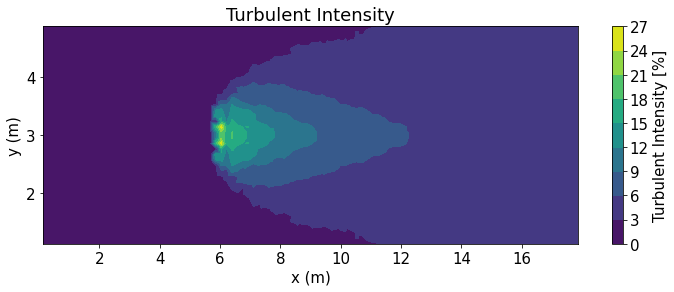
Contour Plot of Turbulent Intensity
Turbulent Intensity is the ratio of the magnitude of turbulent velocity to total velocity. The function turbulent_intensity takes the inputs of the NetCDF object, the points to caculate over, the time index, and an optional boolian input to output intermediate_values used to calculate turbulent intensity. The fuction then pulls variables 'ucx', 'ucy', 'ucz', and 'turkin1' as the velocity in the x, y, waterdepth and turbulence kinetic energy respectively. The function then
calculates and outputs the turbulent intensity, turbulent_intensity, for any given time_index in the data_frame TI. The TI dataframe also includes the x,y, and waterdepth location. If the intermediate_values bollian is equal to true the turbulent kinetic energy 'turkin1', and velocity in the 'ucx', 'ucy', and 'ucz' direction are also included.
In this example it is calculating the turbulent intensity over the same contour_points used above, however it can also calculate over ‘cells’, the coordinate system for the raw velocity data, or ‘faces’, the coordinate system for the raw turbulence data. If nothing is specified for points, 'cells' is the default coordinate system.
Following the same format as the previous two contour plots the limits of the maximum and minimum values are defined by user as well as a string for the type of plot. The code then outputs a contour plot of the turbulent intensity.
[12]:
# Calculating turbulent intensity
TI = d3d.turbulent_intensity(d3d_data, points=contour_points, intermediate_values=True)

# Creating new plot limits
max_plot_TI = 27
min_plot_TI = 0

# Plotting
plt.figure(figsize=(12, 4))
contour_plot = plt.tricontourf(
    TI.x,
    TI.y,
    TI.turbulent_intensity,
    vmin=min_plot_TI,
    vmax=max_plot_TI,
    levels=np.linspace(min_plot_TI, max_plot_TI, 10),
)

plt.xlabel("x (m)")
plt.ylabel("y (m)")
plt.title("Turbulent Intensity")
cbar = plt.colorbar(contour_plot)
cbar.set_label("Turbulent Intensity [%]")

TI
points provided
[12]:
| x | y | waterdepth | turkin1 | ucx | ucy | ucz | turbulent_intensity | |
|---|---|---|---|---|---|---|---|---|
| index | ||||||||
| 0 | 17.875000 | 4.875 | 1.000931 | 0.003148 | 1.115198 | 3.600628e-04 | -0.059917 | 4.101755 |
| 1 | 17.695707 | 4.875 | 1.000931 | 0.003091 | 1.115302 | 3.816327e-04 | 0.079242 | 4.060148 |
| 2 | 17.516414 | 4.875 | 1.000931 | 0.003096 | 1.112163 | 3.603633e-04 | 0.074341 | 4.075892 |
| 3 | 17.337121 | 4.875 | 1.000931 | 0.003013 | 1.108294 | 3.147688e-04 | -0.004829 | 4.043806 |
| 4 | 17.157828 | 4.875 | 1.000931 | 0.003029 | 1.110058 | 2.822649e-04 | -0.012586 | 4.047740 |
| ... | ... | ... | ... | ... | ... | ... | ... | ... |
| 3995 | 0.842172 | 1.125 | 1.000931 | 0.000392 | 1.058136 | -6.727795e-07 | -0.000070 | 1.527464 |
| 3996 | 0.662879 | 1.125 | 1.000931 | 0.000393 | 1.057769 | -4.857739e-07 | 0.011486 | 1.529358 |
| 3997 | 0.483586 | 1.125 | 1.000931 | 0.000399 | 1.059054 | -3.423436e-07 | -0.005860 | 1.540513 |
| 3998 | 0.304293 | 1.125 | 1.000931 | 0.000374 | 1.059019 | -2.209735e-07 | 0.023087 | 1.491256 |
| 3999 | 0.125000 | 1.125 | 1.000931 | 0.000350 | 1.056319 | -1.155897e-07 | 0.135350 | 1.434725 |
4000 rows × 8 columns
Comparing Face Data to Cell Data
In Delft3D there is a staggered grid where some variables are stored on the faces and some are stored on the cells. The d3d.variable_interpolation function allows you to linearly interpolate face data onto the cell locations or vice versa. For this example, we input the variable names, 'ucx', 'ucy','ucz', and 'turkin1', which are pulled from the NetCDF object (d3d_data) and are to be interpolated on to the coordinate system 'faces'. The output is a data frame,
Var, with the interpolated data.
Near the boundaries linear linterpolate will sometimes return negative values. When calculating turbulent intensity negative turbulent kinetic energy values (turkin1) will have and invalid answered. To filter out any negative values the index of where the negative numbers are located are calculated as neg_index. If the value is close to 0 (greater then -1.0e-4) the values is replaced with zero, if not it is replaced with nan. zero_bool determines if the negative number is close to 0.
zero_ind is the location of the negative numbers to be replaced with zero and non_zero_bool are the locations of the numbers to replace with nan. To calculate turbulent intensity the magnitude of the velocity is calculated with 'ucx', 'ucy', 'ucz' and saved as u_mag.Turbulent intensity is then calculated with u_mag and turkin1 and saved as turbulent_intensity.
Linear interpolate can also leave nan values near the edges of data. If you want fill these in using nearest interpolate set the values edges to equal 'nearest' otherwis this option is dufalted to 'none'.
The data can be called, as shown, with Var. We now have 'ucx' and 'turkin1' on the same grid so then can be compared and used in calculations.
[13]:
variables = ["turkin1", "ucx", "ucy", "ucz"]

Var = d3d.variable_interpolation(d3d_data, variables, points="faces", edges="nearest")

# Replacing negative numbers close to zero with zero
neg_index = np.where(Var["turkin1"] < 0)  # Finding negative numbers

# Determining if negative number are close to zero
zero_bool = np.isclose(
    Var["turkin1"][Var["turkin1"] < 0].array,
    np.zeros(len(Var["turkin1"][Var["turkin1"] < 0].array)),
    atol=1.0e-4,
)

# Identifying the location of negative values close to zero
zero_ind = neg_index[0][zero_bool]

# Identifying the location of negative number that are not close to zero
non_zero_ind = neg_index[0][~zero_bool]

# Replacing negative number close to zero with zero
Var.loc[zero_ind, "turkin1"] = np.zeros(len(zero_ind))

# Replacing negative numbers not close to zero with nan
Var.loc[non_zero_ind, "turkin1"] = [np.nan] * len(non_zero_ind)

# Calculating the root mean squared velocity
Var["u_mag"] = d3d.unorm(
    np.array(Var["ucx"]), np.array(Var["ucy"]), np.array(Var["ucz"])
)

# Calculating turbulent intensity as a percent
Var["turbulent_intensity"] = (np.sqrt(2 / 3 * Var["turkin1"]) / Var["u_mag"]) * 100

Var
[13]:
| x | y | waterdepth | turkin1 | ucx | ucy | ucz | u_mag | turbulent_intensity | |
|---|---|---|---|---|---|---|---|---|---|
| index | |||||||||
| 0 | 0.125 | 1.125 | 0.199485 | 0.008562 | 0.717881 | -1.531373e-07 | 0.056840 | 0.720128 | 10.491394 |
| 1 | 0.375 | 1.125 | 0.200008 | 0.008906 | 0.689645 | -3.833700e-07 | -0.011832 | 0.689746 | 11.171384 |
| 2 | 0.125 | 1.375 | 0.199485 | 0.009280 | 0.717881 | -4.313024e-07 | 0.056840 | 0.720128 | 10.922269 |
| 3 | 0.625 | 1.125 | 0.200056 | 0.008780 | 0.694164 | -6.750081e-07 | 0.004593 | 0.694179 | 11.020928 |
| 4 | 0.375 | 1.375 | 0.200008 | 0.008906 | 0.689645 | -1.064686e-06 | -0.011832 | 0.689746 | 11.171384 |
| ... | ... | ... | ... | ... | ... | ... | ... | ... | ... |
| 5755 | 17.625 | 4.625 | 1.794649 | 0.000914 | 1.245117 | 9.389975e-04 | 0.033098 | 1.245558 | 1.982237 |
| 5756 | 17.375 | 4.875 | 1.794848 | 0.000903 | 1.222989 | 2.199022e-04 | 0.000277 | 1.222989 | 2.006523 |
| 5757 | 17.875 | 4.625 | 1.799824 | 0.000908 | 1.255866 | 8.894604e-04 | 0.010782 | 1.255913 | 1.958613 |
| 5758 | 17.625 | 4.875 | 1.794638 | 0.000907 | 1.245292 | 2.690449e-04 | 0.033248 | 1.245736 | 1.973690 |
| 5759 | 17.875 | 4.875 | 1.799828 | 0.000900 | 1.256067 | 2.501023e-04 | 0.011193 | 1.256117 | 1.950496 |
5760 rows × 9 columns
When plotting data using d3d.variable_interpolationit is helpful to define points to interpolate onto as the 'cell' and 'face' grids contain a 3 dimensional grid of points. In this next example we will use the d3d.variable_interpolation function to plot a contour plot of tubulent intesity normal to turbine (y-waterdepth cross section) n turbine diameters downstream of the turbine.
As stated in the intro, the turbine is located at 6m along the length turbine_x_loc with a diameter of 0.7m (turbine_diameter). Similar to the previous example, we input the variable names variables 'ucx', 'ucy','ucz', and 'turkin1', which are pulled from the NetCDF object (d3d_data). Unlike the previous example, the points are defined as sample_points created using create_points from x_sample, y_sample, and waterdepth_sample with
x_sample at a constant point of 1 (N) turbine diameters downstream of the turbine (6.7m) and y_sample and waterdepth_sample being arrays between the minimum and maximum values for that flume dimension. The interpolated data is the saved from d3d.variable_interpolation as Var_sampleand used to calculate turbulent intensity as in the previous example. The data is then plotted along the y and waterdepth axis.
[14]:
turbine_x_loc = 6
turbine_diameter = 0.7
N = 1
x_sample = turbine_x_loc + N * turbine_diameter
y_samples = np.linspace(ymin, ymax, num=40)
waterdepth_samples = np.linspace(waterdepth_min, waterdepth_max, num=256)

variables = ["turkin1", "ucx", "ucy", "ucz"]
sample_points = d3d.create_points(x_sample, y_samples, waterdepth_samples)

Var_sample = d3d.variable_interpolation(
    d3d_data, variables, points=sample_points, edges="nearest"
)

# root mean squared calculation
Var_sample["u_mag"] = d3d.unorm(
    np.array(Var_sample["ucx"]),
    np.array(Var_sample["ucy"]),
    np.array(Var_sample["ucz"]),
)
# turbulent intesity calculation
Var_sample["turbulent_intensity"] = (
    np.sqrt(2 / 3 * Var_sample["turkin1"]) / Var_sample["u_mag"] * 100
)

# Plotting
plt.figure(figsize=(10, 4.4))
contour_plot = plt.tricontourf(
    Var_sample.y,
    Var_sample.waterdepth,
    Var_sample.turbulent_intensity,
    vmin=min_plot_TI,
    vmax=max_plot_TI,
    levels=np.linspace(min_plot_TI, max_plot_TI, 10),
)

plt.xlabel("y (m)")
plt.ylabel("z (m)")
plt.title("Turbulent Intensity")
cbar = plt.colorbar(contour_plot)
cbar.set_label("Turbulent Intensity [%]")
points provided
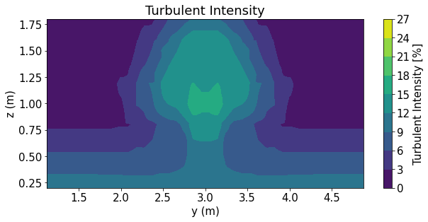
This sample data used in this example is not spatial or temporally resolved and is for demonstration purposes only. In this example there are 5 sigma layers. The low level of discretization can be seen in in the sharp edges in the turbulent intensity plot above around the turbine.
[ ]: