MHKiT Environmental Contours

Environmental contours of extreme sea states can be used as a part of reliability-based design for offshore structures, including wave energy converters (WECs). Environmental contours provide estimations of extreme sea states based on short-term data (e.g. 10 years used to estimate a 100-year event). These environmental contours describe extreme sea states by characterizing the resource, defining sea states for extreme condition analysis, and developing a framework for analyzing survivability of a design.

MHKiT includes functions adapted from the WDRT for creating environmental contours of extreme sea states using a principal component analysis (PCA) methodology, with additional improvements for characterizing the joint probability distribution of sea states. As a demonstration, this notebook will walk through the following steps to find a 100-year sea state for NDBC buoy 46022 using 16 years of spectral wave density data.

1. Request Spectral Wave Density Data from NDBC

2. Calculate Hm0 and Te using the requested data

3. Find the data’s 100-year contour

4. Plot the data and the 100-year contour

We will start by importing the necessary python packages (scipy, pandas, numpy), and MHKiT wave submodules (resource, contours, graphics, and io.ndbc).

from mhkit.wave import resource, contours, graphics
import matplotlib.pyplot as plt
from mhkit.wave.io import ndbc
from scipy import stats
import pandas as pd
import numpy as np

1. Request Spectral Wave Density Data from NDBC

MHKiT can be used to request historical data from the National Data Buoy Center (NDBC). This process is split into the following steps:

• Query available NDBC data

• Select years of interest

• Request Data from NDBC

• Convert the DataFrames to DateTime Index

Query available NDBC data

Looking at the help for the ndbc.available_data function (help(ndbc.available_data)) the function requires a parameter to be specified and optionally the user may provide a station ID as a string. A full list of available historical parameters can be found here although only some of these are currently supported. We are interested in historical spectral wave density data 'swden' (from which we may calculate Hm0 and Te). Additionally, we will specify the buoy number as '46022' to only return data associated with this site.

# Specify the parameter as spectral wave density and the buoy number to be 46022
parameter = "swden"
buoy_number = "46022"
ndbc_available_data = ndbc.available_data(parameter, buoy_number)
ndbc_available_data.head()

	id	year	filename
1658	46022	1996	46022w1996.txt.gz
1659	46022	1997	46022w1997.txt.gz
1660	46022	1998	46022w1998.txt.gz
1661	46022	1999	46022w1999.txt.gz
1662	46022	2000	46022w2000.txt.gz

Select years of interest

The ndbc.available_data function has returned a DataFrame with columns ‘id’, ‘year’, and ‘filename’. The year column is of type int while the filename and id (5 digit alpha-numeric specifier) are of type string. In this case, the years returned from ndbc_available_data span 1996 to the last complete year the buoy was operational (currently 2019 for 46022). For demonstration, we have decided we are interested in the data between the years 1996 and 2012 so we will create a new years_of_interest DataFrame which only contains years less than 2013.

# Slice the available data to only include through year 2012
years_of_interest = ndbc_available_data[ndbc_available_data.year < 2013]
years_of_interest.head()

	id	year	filename
1658	46022	1996	46022w1996.txt.gz
1659	46022	1997	46022w1997.txt.gz
1660	46022	1998	46022w1998.txt.gz
1661	46022	1999	46022w1999.txt.gz
1662	46022	2000	46022w2000.txt.gz

Request Data from NDBC

The filename column in our years_of_interest DataFrame and the parameter is needed to request the data. To get the data we can use the ndbc.request_data function to iterate over each buoy id and year in the passed DataFrame. This function will return the parameter data as a dictionary of DataFrames which may be accessed by buoy id and then the year for multiple buoys or just the year for a single buoy.

# Get dictionary of parameter data by year
filenames = years_of_interest["filename"]
ndbc_requested_data = ndbc.request_data(parameter, filenames)

Convert the DataFrames to DateTime Index

The data returned for each year has a variable number of columns for the year, month, day, hour, minute, and the way the columns are formatted (this is a primary reason for return a dictionary of DataFrames indexed by years). A common step a user will want to take is to remove the inconsistent NDBC date/ time columns and create a standard DateTime index. The MHKiT function ndbc.to_datetime_index will perform this standardization by parsing the NDBC date/ time columns into DateTime format and setting this as the DataFrame Index and removing the NDBC date/ time columns. This function operates on a DateFrame therefore we will iterate over each year of the ndbc_requested_data dictionary.

# Lastly we will convert a DateTime Index
ndbc_data = {}
# Create a Datetime Index and remove NOAA date columns for each year
for year in ndbc_requested_data:
    year_data = ndbc_requested_data[year]
    ndbc_data[year] = ndbc.to_datetime_index(parameter, year_data)

# Display DataFrame of 46022 data from 1996
ndbc_data["1996"].head()

	0.03	0.04	0.05	0.06	0.07	0.08	0.09	0.10	0.11	0.12	...	0.31	0.32	0.33	0.34	0.35	0.36	0.37	0.38	0.39	0.40
date
1996-01-01 00:00:00	0.0	2.11	27.49	41.63	27.23	17.09	8.61	5.05	3.73	2.82	...	0.17	0.16	0.14	0.15	0.13	0.09	0.09	0.08	0.06	0.06
1996-01-01 01:00:00	0.0	1.20	25.13	57.69	32.59	11.75	6.33	4.16	4.22	2.98	...	0.22	0.18	0.20	0.10	0.12	0.10	0.07	0.07	0.05	0.04
1996-01-01 02:00:00	0.0	0.90	15.98	48.98	37.98	23.56	11.87	6.80	3.75	3.00	...	0.14	0.15	0.20	0.12	0.08	0.08	0.07	0.09	0.07	0.05
1996-01-01 03:00:00	0.0	0.38	14.73	38.55	34.99	14.79	9.23	5.54	4.43	2.99	...	0.17	0.20	0.17	0.14	0.12	0.09	0.07	0.05	0.06	0.04
1996-01-01 04:00:00	0.0	0.12	22.77	52.11	34.88	18.90	13.36	7.49	2.94	2.55	...	0.12	0.11	0.09	0.13	0.10	0.08	0.08	0.07	0.03	0.03

5 rows × 38 columns

2. Calculate \(H_{m0}\) and \(T_e\) using the NDBC Data

A sea state may be characterized by significant wave height (Hm0) and energy period (Te). Using the historical spectral wave density data from NDBC, we can calculate these variables using MHKiT. Both Hm0 and Te return a single value for a given time (e.g. DateTime index). Currently, the data remains as a dictionary of DataFrames because the frequency binning (range and discretization) change across years of NDBC data. Once we have a single value for each DateTime we can combine all the data into a single DataFrame.

# Intialize empty lists to store the results from each year
Hm0_list = []
Te_list = []

# Iterate over each year and save the result in the initalized dictionary
for year in ndbc_data:
    year_data = ndbc_data[year]
    Hm0_list.append(resource.significant_wave_height(year_data.T))
    Te_list.append(resource.energy_period(year_data.T))

# Concatenate each list of Series into a single Series
Te = pd.concat(Te_list, axis=0)
Hm0 = pd.concat(Hm0_list, axis=0)

# Name each Series and concat into a dataFrame
Te.name = 'Te'
Hm0.name = 'Hm0'
Hm0_Te = pd.concat([Hm0, Te], axis=1)

# Drop any NaNs created from the calculation of Hm0 or Te
Hm0_Te.dropna(inplace=True)
# Sort the DateTime index
Hm0_Te.sort_index(inplace=True)
Hm0_Te

	Hm0	Te
index
1996-01-01 00:00:00	4.819627	14.856398
1996-01-01 01:00:00	5.004158	14.961679
1996-01-01 02:00:00	5.091169	14.244618
1996-01-01 03:00:00	4.679487	14.042246
1996-01-01 04:00:00	5.140895	14.478961
...	...	...
2012-12-31 19:00:00	1.995194	14.757854
2012-12-31 20:00:00	1.976259	14.360242
2012-12-31 21:00:00	2.658421	15.708162
2012-12-31 22:00:00	2.364910	15.247587
2012-12-31 23:00:00	2.056891	14.328179

125410 rows × 2 columns

3. Find the contour line for the 100 year

With the sea state data calculated, we can now use the modified I-FORM method to define reliability for a 100-year sea state based on the 17 years of spectral wave density data obtained from NDBC for buoy 46022. Reliability is the likelihood that a certain event will not occur in a given period. The period will define a line of constant probability in the joint probability of \(H_{m0}\) and \(T_e\) but individually each component different reliability (marginal distribution) which we can find by evaluating a normal cumulative distribution function (CDF). This CDF returns each component’s quantiles along the iso-reliability line that finally allows us to calculate each sea state value (e.g. the 100-year contour values for Hm0 and Te).

For more detail on the environmental contour method used here please refer to: Eckert-Gallup et. al 2016

To apply the environmental_contours function we will specify a 100-year sea state, the sea state data (Hm0, Te), and the time difference between measurements (dt in seconds).

# Return period (years) of interest
period = 100

# Remove Hm0 Outliers
Hm0_Te_clean = Hm0_Te[Hm0_Te.Hm0 < 20]

# Get only the values from the DataFrame
Hm0 = Hm0_Te_clean.Hm0.values
Te = Hm0_Te_clean.Te.values

# Delta time of sea-states
dt = (Hm0_Te_clean.index[2] - Hm0_Te_clean.index[1]).seconds

# Get the contour values
copula = contours.environmental_contours(Hm0, Te, dt, period, "PCA", return_PCA=True)
Hm0_contour = copula["PCA_x1"]
Te_contour = copula["PCA_x2"]

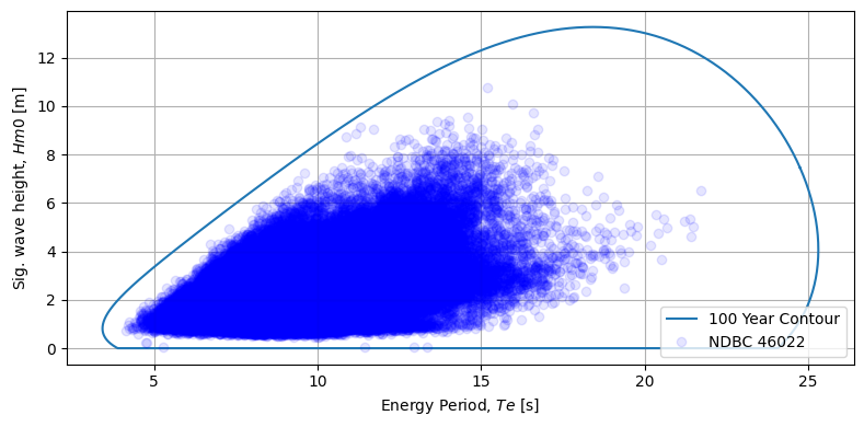
4. Plot overlay of the data and contour

Lastly we can use the MHKiT graphics module to create a contour plot which shows the data and resultant conotour line.

fig, ax = plt.subplots(figsize=(8, 4))
# %matplotlib inline
ax = graphics.plot_environmental_contour(
    Te,
    Hm0,
    Te_contour,
    Hm0_contour,
    data_label="NDBC 46022",
    contour_label="100 Year Contour",
    x_label="Energy Period, $Te$ [s]",
    y_label="Sig. wave height, $Hm0$ [m]",
    ax=ax,
)

Other Contour Methods

MHKiT has parametric, nonparametric, and Kernel Density Estimation methods for calculating environmental contours housed within the resource.environmental_contours function. We can compare other copulas to our PCA method simply by adding more methods. A single string method can be applied if only one copula is of interest as was done above for the PCA method or multiple methods can be sent in using a list of strings. If mutiple methods of the same type are desired is recommended to run them at the same time if possible as it will reduce the computational expense by utilizing the common computational calls across the copulas. In the example below we will compare the parametric and nonparametric Gaussain contours to the PCA method we ran previously.

We start by using the default settings for our Gaussian methods. The environmental_contours function returns a dictionary with component ‘x1’ and ‘x2’ for each method. E.g. if the environmental_contours function were called with the 'gaussian' method then environmental_contours function would return a dictionary with keys ['gaussian_x1', 'gaussian_x2']. The copula methods are a generalized mathematical method and therefore ‘x1’ and ‘x2’ are used in place of Hm0 and Te for the component values. ‘x1’ refers to the first array passed and ‘x2’ refers to the second array passed. In the example below ‘x1’ would refer to the Hm0 component of the coupla and ‘x2’ would refer to Te.

copulas = contours.environmental_contours(
    Hm0, Te, dt, period, method=["gaussian", "nonparametric_gaussian"]
)

fig, ax = plt.subplots(figsize=(9, 4))

Tes = [Te_contour]
Hm0s = [Hm0_contour]
methods = ["gaussian", "nonparametric_gaussian"]
for method in methods:
    Hm0s.append(copulas[f"{method}_x1"])
    Tes.append(copulas[f"{method}_x2"])

ax = graphics.plot_environmental_contour(
    Te,
    Hm0,
    Tes,
    Hm0s,
    data_label="NDBC 46050",
    contour_label=["PCA", "Gaussian", "Nonparametric Gaussian"],
    x_label="Energy Period, $Te$ [s]",
    y_label="Sig. wave height, $Hm0$ [m]",
    ax=ax,
)

Resource Clusters

Often in resource characterization we want to pick a few representative sea state to run an alaysis. To do this with the resource data in python we reccomend using a Gaussian Mixture Model (a more generalized k-means clustering method). Using sckitlearn this is very straight forward. We combine our Hm0 and Te data into an N x 2 numpy array. We specify our number of components (number of representative sea states) and then call the fit method on the data. Fianlly, using the methods means_ and weights we can organize the results into an easily digestable table.

# Intialize empty lists to store the results from each year
Hm0_list = []
Tp_list = []

# Iterate over each year and save the result in the initalized dictionary
for year in ndbc_data:
    year_data = ndbc_data[year]
    Hm0_list.append(resource.significant_wave_height(year_data.T))
    Tp_list.append(resource.peak_period(year_data.T))

# Concatenate each list of Series into a single Series
Tp = pd.concat(Tp_list, axis=0)
Hm0 = pd.concat(Hm0_list, axis=0)

# Name each Series and concat into a dataFrame
Tp.name = 'Tp'
Hm0.name = 'Hm0'
Hm0_Tp = pd.concat([Hm0, Tp], axis=1)

# Drop any NaNs created from the calculation of Hm0 or Te
Hm0_Tp.dropna(inplace=True)
# Sort the DateTime index
Hm0_Tp.sort_index(inplace=True)

# Remove Hm0 Outliers
Hm0_Tp_clean = Hm0_Tp[Hm0_Tp.Hm0 < 20]
Hm0_Tp_clean = Hm0_Tp[Hm0_Tp.Tp < 30]

# Get only the values from the DataFrame
Hm0 = Hm0_Tp_clean.Hm0.values
Tp = Hm0_Tp_clean.Tp.values


Hm0_Tp

	Hm0	Tp
index
1996-01-01 00:00:00	4.819627	16.666667
1996-01-01 01:00:00	5.004158	16.666667
1996-01-01 02:00:00	5.091169	16.666667
1996-01-01 03:00:00	4.679487	16.666667
1996-01-01 04:00:00	5.140895	16.666667
...	...	...
2012-12-31 19:00:00	1.995194	19.047619
2012-12-31 20:00:00	1.976259	17.391304
2012-12-31 21:00:00	2.658421	17.391304
2012-12-31 22:00:00	2.364910	17.391304
2012-12-31 23:00:00	2.056891	17.391304

125426 rows × 2 columns

from sklearn.mixture import GaussianMixture

# Compute Gaussian Mixture Model
X = np.vstack((Tp, Hm0)).T
gmm = GaussianMixture(n_components=8).fit(X)

# Save centers and weights
results = pd.DataFrame(gmm.means_, columns=["Tp", "Hm0"])
results["weights"] = gmm.weights_
results

	Tp	Hm0	weights
0	7.529565	1.595490	0.182459
1	12.115343	2.669366	0.219278
2	16.567481	2.636207	0.073010
3	10.216278	1.743338	0.160776
4	13.455188	4.738885	0.041351
5	8.692400	2.779776	0.171362
6	19.900045	2.707808	0.018114
7	14.290462	2.808907	0.133650

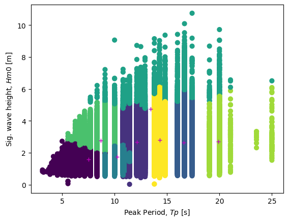
Viewing the Clusters

We can visually look at the clusters by predicting which cluster each datapoint belongs in. Then we can plot the means on top of this to show where each cluster is centered and how the data points are being catagorized.

# Plot the Sections of Data
labels = gmm.predict(X)
plt.scatter(Tp, Hm0, c=labels, s=40)
plt.plot(results.Tp, results.Hm0, "m+")
plt.xlabel("Peak Period, $Tp$ [s]")
plt.ylabel("Sig. wave height, $Hm0$ [m]")

Text(0, 0.5, 'Sig. wave height, $Hm0$ [m]')