MHKiT WEC-Sim Example

This example loads simulated data from a WEC-Sim run for a two-body point absorber (Reference Model 3) and demonstrates the application of the MHKiT wave module to interact with the simulated data. The analysis is broken down into three parts: load WEC-Sim data, view and interact with the WEC-Sim data , and apply the MHKiT wave module.

1. Load WEC-Sim Simulated Data

2. WEC-Sim Simulated Data

   • Wave Class Data

   • Body Class Data

   • PTO Class Data

   • Constraint Class Data

   • Mooring Class Data

3. Apply MHKiT Wave Module

Start by importing MHKiT and the necessary python packages (e.g.scipy.io and matplotlib.pyplot).

from  mhkit import wave
import scipy.io as sio
import matplotlib.pyplot as plt

1. Load WEC-Sim Simulated Data

WEC-Sim saves output data as a MATLAB output object, generated by WEC-Sim’s Response Class. The WEC-Sim output object must be converted to a structure for use in Python.

Here we will load the WEC-Sim RM3 data run with a mooring matrix.

# Relative location and filename of simulated WEC-Sim data (run with mooring)
filename = './data/wave/RM3MooringMatrix_matlabWorkspace_structure.mat'

# Load data using the `wecsim.read_output` function which returns a dictionary of dataFrames
wecsim_data = wave.io.wecsim.read_output(filename)

moorDyn class not used
ptosim class not used
cable class not used

NOTE: The mhkit.wave.io.wecsim.read_output function prints a message letting the user know which WEC-Sim classes were not used. This WEC-Sim example data for the RM3 was not run with MoorDyn, PTO-Sim or a cable.

NOTE: Conversion of the WEC-Sim object to a struct must be done in MATLAB and can be achieved using the command: output = struct(output);.

2. WEC-Sim Simulated Data

This section will investigate the WEC-Sim RM3 data loaded using MHKiT. In the previous section mhkit.wave.io.wecsim.read_output returned a dictonary of DataFrames in a format similar to the WEC-Sim output object. To see what data is available we can call the keys method on the wecsim_data dictionary:

# View the available WEC-Sim data, a dataFrame for each WEC-Sim Class
wecsim_data.keys()

dict_keys(['wave', 'bodies', 'ptos', 'constraints', 'mooring', 'moorDyn', 'ptosim', 'cables'])

We can see above that there are eight returned keys. As noted from the mhkit.wave.io.wecsim.read_output function the moorDyn, ptosim and cables keys will be empty as the function found the data missing from the output. The following sections will work through each of the 5 other WEC-Sim classes.

Wave Class Data

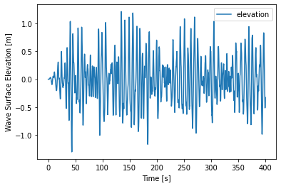
Data from WEC-Sim’s Wave Class includes information about the wave input, including the the wave type, and wave elevation as a function of time. Below we will wave the wave DataFrame as wave and then look at the wave type and the top (head) of the DataFrame.

# Store WEC-Sim output from the Wave Class to a new dataFrame, called `wave_data`
wave_data = wecsim_data['wave']

# Display the wave type from the WEC-Sim Wave Class
wave_type = wave_data.name
print("WEC-Sim wave type:", wave_type)

# View the WEC-Sim output dataFrame for the Wave Class
wave_data

WEC-Sim wave type: elevationImport

	elevation
time
0.00	-0.000000e+00
0.01	-2.766568e-07
0.02	-1.106006e-06
0.03	-2.486738e-06
0.04	-4.416811e-06
...	...
399.96	-3.480172e-01
399.97	-3.429291e-01
399.98	-3.378586e-01
399.99	-3.326988e-01
400.00	-3.274562e-01

40001 rows × 1 columns

The WEC-Sim wave type refers to the type of wave used to run the WEC-Sim simulation. Data from this WEC-Sim run was generated used ‘etaImport’, meaning a user-defined wave surface elevation was defined. For more information about the wave types used by WEC-Sim, refer to the Wave Class documentation.

Plot the Wave Elevation Data

We can use the pandas DataFrame plot method to quickly view the Data. The plot method will set the index (time) on the x-axis and any columns (in this case only wave elevation) on the y-axis.

# Plot WEC-Sim output from the Wave Class
wave_data.plot()
plt.xlabel("Time [s]")
plt.ylabel("Wave Surface Elevation [m]")

Text(0, 0.5, 'Wave Surface Elevation [m]')

Body Class Data

Data from WEC-Sim’s Body Class includes information about each body, including the body’s position, velocity, acceleration, forces acting on the body, and the body’s name. For the RM3 example there will be 2 boides a float and a spar.

# Store WEC-Sim output from the Body Class to a new dictionary of dataFrames, i.e. 'bodies'.
bodies = wecsim_data['bodies']

# Data fron each body is stored as its own dataFrame, i.e. 'body1' and 'body2'.
bodies.keys()

dict_keys(['body1', 'body2'])

Body Class Data for Body 1

Let us determine which body ‘body1’ is by requesting the body’s name. In this this case the body name is ‘float’.

# Store Body Class dataFrame for Body 1 as `body1`.
body1 = bodies['body1']

# Display the name of Body 1 from the WEC-Sim Body Class
print("Name of Body 1:", body1.name)

Name of Body 1: float

For a given body WEC-Sim returns simulated parameters (the number of simulated parameters varies by the options choosen) for each of the 6 degrees of freedom (DOF). We can view the unique simulated parameters by filtering the columns by a single DOF. For this example we look at surge data (DOF 1).

# Print a list of Body 1 columns that end with 'dof1'
[col for col in body1 if col.endswith('dof1')]

['position_dof1',
 'velocity_dof1',
 'acceleration_dof1',
 'forceTotal_dof1',
 'forceExcitation_dof1',
 'forceRadiationDamping_dof1',
 'forceAddedMass_dof1',
 'forceRestoring_dof1',
 'forceMorisonAndViscous_dof1',
 'forceLinearDamping_dof1']

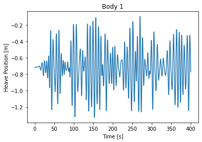
Plot heave position data for Body 1

The RM3 device creates power in the heave direction (DOF 3). Let us consider the float’s (body 1) position as a function of time by plotting postion_dof3.

# Use Pandas to plot Body 1 position in heave (DOF 3)
body1.position_dof3.plot()
plt.xlabel("Time [s]")
plt.ylabel("Heave Position [m]")
plt.title('Body 1')

# Use Pandas to calculate the maximum and minimum heave position of Body 1
print("Body 1 max heave position =", body1.position_dof3.max(),"[m]")
print("Body 1 min heave position =", body1.position_dof3.min(),"[m]")

Body 1 max heave position = -0.09745294999054366 [m]
Body 1 min heave position = -1.3264489287377081 [m]

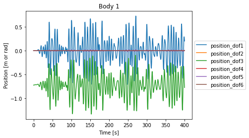
Plot Body 1 position data for all DOFs

As an example we could plot multiple postion DOFs by calling a plot on only the position columns. To do that we would first create a list of stings (filter_col) which include the string 'position'. Then slicing the DataFrame on that list of strings and calling plot will plot the position over time of all 6 degrees of freedom for body1.

# Create a list of Body 1 data columns that start with 'position'
filter_col = [col for col in body1 if col.startswith('position')]

# Plot filtered 'position' data for Body 1
body1[filter_col].plot()
plt.xlabel('Time [s]')
plt.ylabel('Position [m or rad]')
plt.title('Body 1')
plt.legend(loc='center left', bbox_to_anchor=(1, 0.5))

<matplotlib.legend.Legend at 0x204dea0fdf0>

Body Class Data for Body 2

We can look at the name of body 2 to see that is the ‘sapr’ of RM3. Looking at the top of the body2 DataFrame we see the same available data as body1.

# Store Body Class dataFrame for Body 2 as `body2`
body2 = bodies['body2']

# Display the name of Body 2 from the WEC-Sim Body Class
print("Name of Body 2:", body2.name)

# View the Body Class dataFrame for Body 2
body2.head()

Name of Body 2: spar

	position_dof1	velocity_dof1	acceleration_dof1	forceTotal_dof1	forceExcitation_dof1	forceRadiationDamping_dof1	forceAddedMass_dof1	forceRestoring_dof1	forceMorisonAndViscous_dof1	forceLinearDamping_dof1	...	position_dof6	velocity_dof6	acceleration_dof6	forceTotal_dof6	forceExcitation_dof6	forceRadiationDamping_dof6	forceAddedMass_dof6	forceRestoring_dof6	forceMorisonAndViscous_dof6	forceLinearDamping_dof6
time
0.00	0.000000e+00	0.000000e+00	3.755268e-11	0.002335	0.000000	0.0	-0.002335	0.0	0	0	...	0.0	0.0	0.0	-0.000032	0.000000e+00	0.0	0.000032	0.0	0	0
0.01	1.591394e-14	3.896569e-12	4.658216e-10	0.003717	0.000114	0.0	-0.003603	0.0	0	0	...	0.0	0.0	0.0	-0.000049	3.542912e-11	0.0	0.000049	0.0	0	0
0.02	1.060269e-13	1.600503e-11	1.593218e-09	0.005343	0.000471	0.0	-0.004872	0.0	0	0	...	0.0	0.0	0.0	-0.000068	1.419347e-10	0.0	0.000068	0.0	0	0
0.03	3.850573e-13	4.276107e-11	3.369237e-09	0.006388	0.001097	0.0	-0.005291	0.0	0	0	...	0.0	0.0	0.0	-0.000079	3.198299e-10	0.0	0.000079	0.0	0	0
0.04	1.024419e-12	8.867535e-11	5.507643e-09	0.006671	0.002016	0.0	-0.004656	0.0	0	0	...	0.0	0.0	0.0	-0.000081	5.694090e-10	0.0	0.000081	0.0	0	0

5 rows × 60 columns

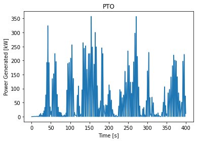
PTO Class Data

Data from WEC-Sim’s PTO Class includes information about each PTO, including the PTO’s position, velocity, acceleration, forces acting on the PTO, and the PTO’s name. In this case there is only 1 PTO.

# Store WEC-Sim output from the PTO Class to a DataFrame, called `ptos`
ptos = wecsim_data['ptos']

# Display the name of the PTO from the WEC-Sim PTO Class
print("Name of PTO:", ptos.name)

# Print a list of available columns that end with 'dof1'
[col for col in ptos if col.endswith('dof1')]

Name of PTO: PTO1

['position_dof1',
 'velocity_dof1',
 'acceleration_dof1',
 'forceTotal_dof1',
 'forceActuation_dof1',
 'forceConstraint_dof1',
 'forceInternalMechanics_dof1',
 'powerInternalMechanics_dof1']

# Use Pandas to plot pto internal power in heave (DOF 3)
# NOTE: WEC-Sim requires a negative sign to convert internal power to generated power
(-1*ptos.powerInternalMechanics_dof3/1000).plot()
plt.xlabel("Time [s]")
plt.ylabel("Power Generated [kW]")
plt.title('PTO')

Text(0.5, 1.0, 'PTO')

Constraint Class Data

Data from WEC-Sim’s Constraint Class includes information about each constraint, including the constraint’s position, velocity, acceleration, forces acting on the constraint, and the constraint’s name.

# Store WEC-Sim output from the Constraint Class to a new dataFrame, called `constraints`
constraints = wecsim_data['constraints']

# Display the name of the Constraint from the WEC-Sim Constraint Class
print("Name of Constraint:", constraints.name)

# View the Constraint Class dataFrame
constraints.head()

Name of Constraint: Constraint1

	position_dof1	velocity_dof1	acceleration_dof1	forceConstraint_dof1	position_dof2	velocity_dof2	acceleration_dof2	forceConstraint_dof2	position_dof3	velocity_dof3	...	acceleration_dof4	forceConstraint_dof4	position_dof5	velocity_dof5	acceleration_dof5	forceConstraint_dof5	position_dof6	velocity_dof6	acceleration_dof6	forceConstraint_dof6
time
0.00	0.000000e+00	0.000000e+00	-2.382256e-10	0.0	0.0	0.0	0.0	1.615587e-27	0.000000e+00	0.000000	...	0.0	-3.636025	-0.000000e+00	-0.000000e+00	-1.282689e-11	-0.0	0.0	0.0	0.0	-7.703720e-34
0.01	-7.759428e-14	-1.900049e-11	-2.327210e-09	0.0	0.0	0.0	0.0	1.198363e-03	1.828372e-07	0.000039	...	0.0	-3.325180	-4.349220e-15	-1.064980e-12	-1.299084e-10	-0.0	0.0	0.0	0.0	3.168962e-05
0.02	-4.942732e-13	-7.203815e-11	-6.948927e-09	0.0	0.0	0.0	0.0	2.493818e-03	8.204028e-07	0.000091	...	0.0	-2.984545	-2.792094e-14	-4.095032e-12	-3.973091e-10	-0.0	0.0	0.0	0.0	6.653122e-05
0.03	-1.677273e-12	-1.739122e-10	-1.255916e-08	0.0	0.0	0.0	0.0	3.245134e-03	2.036966e-06	0.000154	...	0.0	-2.781700	-9.592234e-14	-1.007783e-11	-7.408555e-10	-0.0	0.0	0.0	0.0	8.740994e-05
0.04	-4.117573e-12	-3.216348e-10	-1.705139e-08	0.0	0.0	0.0	0.0	3.345214e-03	3.906281e-06	0.000220	...	0.0	-2.746425	-2.391624e-13	-1.908419e-11	-1.049258e-09	-0.0	0.0	0.0	0.0	9.123989e-05

5 rows × 24 columns

Mooring Class Data

Data from WEC-Sim’s Mooring Class includes relevant information about the mooring, including the mooring’s position, velocity, mooring force, and the mooring’s name.

# Store WEC-Sim output from the Mooring Class to a new dataFrame, called `mooring`
mooring = wecsim_data['mooring']

# View the PTO Class dataFrame
mooring.head()

	position_dof1	velocity_dof1	forceMooring_dof1	position_dof2	velocity_dof2	forceMooring_dof2	position_dof3	velocity_dof3	forceMooring_dof3	position_dof4	velocity_dof4	forceMooring_dof4	position_dof5	velocity_dof5	forceMooring_dof5	position_dof6	velocity_dof6	forceMooring_dof6
time
0.00	0.000000e+00	0.000000e+00	0.000000e+00	0.0	0.0	0.0	0.000000e+00	0.000000	0.0	0.0	0.0	0.0	-0.000000e+00	-0.000000e+00	0.0	0.0	0.0	0.0
0.01	-7.759428e-14	-1.900049e-11	7.759428e-09	0.0	0.0	0.0	1.828372e-07	0.000039	0.0	0.0	0.0	0.0	-4.349220e-15	-1.064980e-12	0.0	0.0	0.0	0.0
0.02	-4.942732e-13	-7.203815e-11	4.942732e-08	0.0	0.0	0.0	8.204028e-07	0.000091	0.0	0.0	0.0	0.0	-2.792094e-14	-4.095032e-12	0.0	0.0	0.0	0.0
0.03	-1.677273e-12	-1.739122e-10	1.677273e-07	0.0	0.0	0.0	2.036966e-06	0.000154	0.0	0.0	0.0	0.0	-9.592234e-14	-1.007783e-11	0.0	0.0	0.0	0.0
0.04	-4.117573e-12	-3.216348e-10	4.117573e-07	0.0	0.0	0.0	3.906281e-06	0.000220	0.0	0.0	0.0	0.0	-2.391624e-13	-1.908419e-11	0.0	0.0	0.0	0.0

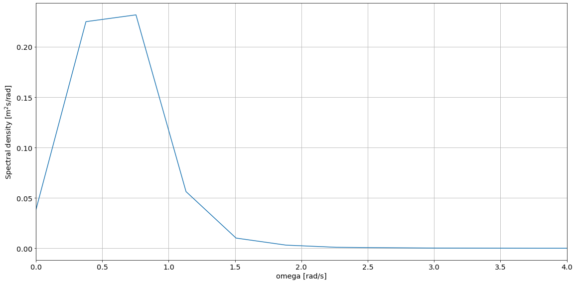
3. Apply MHKiT Wave Module

In the example below we will calculate a spectrum from the wecsim wave elevation timeseries data using the MHKiT elevation_spectrum function.

# Use the MHKiT Wave Module to calculate the wave spectrum from the WEC-Sim Wave Class Data
sample_rate=60
nnft=1000        # Number of bins in the Fast Fourier Transform
ws_spectrum = wave.resource.elevation_spectrum(wave_data, sample_rate, nnft)

# Plot calculated wave spectrum
spect_plot = wave.graphics.plot_spectrum(ws_spectrum)
spect_plot = spect_plot.set_xlim([0, 4])

# Calculate Peak Wave Period (Tp) and Significant Wave Height (Hm0)
Tp = wave.resource.peak_period(ws_spectrum)
Hm0 = wave.resource.significant_wave_height(ws_spectrum)

# Display calculated Peak Wave Period (Tp) and Significant Wave Height (Hm0)
display(Tp,Hm0)

	Tp
elevation	8.333333

	Hm0
elevation	1.785851