ADCP Discharge Example
This example notebook overviews how to calculate discharge from an ADCP transect. The example data used in this notebook was taken by a Teledyne RDI RiverPro ADCP, an instrument purpose-built for calculating discharge from a survey transect, but the following workflow can be used with any ADCP’s data, given that there is GPS information and/or bottom track measurements stored in the ADCP file.
The basic steps that the notebook conducts are to 1. Read in the binary ADCP file 2. Rotate the dataset into the Earth coordinate system (“East”, “North”, “Up”) 3. Correct vessel motion using stored bottom track (You can also use the GPS’s velocity measurement, found from the VTG sentence and converted from speed and direction to velocity-east and velocity-north) 4. Rotate the dataset into the water current’s principal coordinate system (“streamwise”, “cross-stream”, “vertical”) 5. Calculate the distance from the ADCP to the riverbed/seabed. (We use the bottom track ping here, but can also use the ADCP’s altimeter, if available) 6. Finally, calculate the water discharge. Additional parameters that are not availble within the ADCP’s dataset are required here.
We’ll start by immediately jumping through steps 1 and 2. Note if that quality control is required, that should be done here.
[1]:
from mhkit import dolfyn

ds = dolfyn.read_example("RiverPro_test01.PD0")
ds.velds.set_declination(18)  # Set declination to 18 degrees East
ds.velds.rotate2("earth")

# # Note, if the range coordinate has not been adjusted given the depth of the ADCP
# # below the waterline, do so using the following line.
# ds = dolfyn.adp.clean.set_range_offset(ds, x.x)  # Set range offset to x.x m
Reading file c:\users\mcve343\mhkit-python\examples\data\dolfyn/RiverPro_test01.PD0 ...
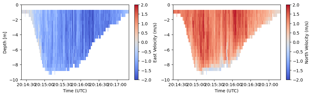
We can plot the dataset below so we know what we are looking at
[2]:
import matplotlib.pyplot as plt

fig, ax = plt.subplots(1,2, figsize=(10,3), constrained_layout=True)
e = ax[0].pcolormesh(ds["time"].values, -ds["range"].values, ds["vel"][0], cmap="coolwarm", vmin=-2, vmax=2)
n = ax[1].pcolormesh(ds["time"].values, -ds["range"].values, ds["vel"][1], cmap="coolwarm", vmin=-2, vmax=2)
fig.colorbar(e, ax=ax[0], label="East Velocity (m/s)")
fig.colorbar(n, ax=ax[1], label="North Velocity (m/s)")
for a in ax:
    a.set(xlabel="Time (UTC)", ylim=(-10, 0))
ax[0].set(ylabel="Depth [m]")
[2]:
[Text(0, 0.5, 'Depth [m]')]
The next step we need to do is to make sure we correct the ADCP measurement for the vessel motion. This is not done natively in the raw ADCP file.
[3]:
# Correct velocity
ds["vel_bt"] = ds["vel_bt"].where((ds["vel_bt"] < 5) & (ds["vel_bt"] > -5))
ds["vel"] -= ds["vel_bt"]
Then rotate into principal coordinates.
[4]:
# Rotate to principal reference frame
ds.attrs["principal_heading"] = dolfyn.calc_principal_heading(ds["vel"].mean("range"))
ds.velds.rotate2("principal")
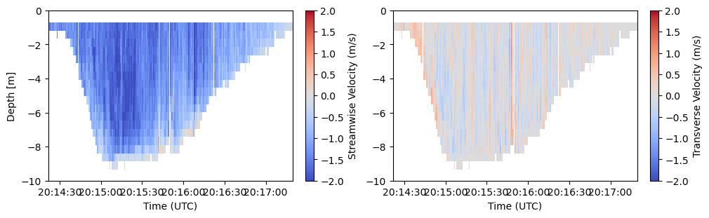
And replot…
The sign associated with the streamwise velocity is a byproduct of the principal direction calculation; it should be associated with ebb or flood tide based on visual observation. The sign associated with the cross-stream (transverse) velocity is related to the streamwise velocity by the right-hand-rule.
[5]:
fig, ax = plt.subplots(1,2, figsize=(10,3), constrained_layout=True)
s = ax[0].pcolormesh(ds["time"].values, -ds["range"].values, ds["vel"][0], cmap="coolwarm", vmin=-2, vmax=2)
t = ax[1].pcolormesh(ds["time"].values, -ds["range"].values, ds["vel"][1], cmap="coolwarm", vmin=-2, vmax=2)
fig.colorbar(s, ax=ax[0], label="Streamwise Velocity (m/s)")
fig.colorbar(t, ax=ax[1], label="Transverse Velocity (m/s)")
for a in ax:
    a.set(xlabel="Time (UTC)", ylim=(-10, 0))
ax[0].set(ylabel="Depth [m]")
[5]:
[Text(0, 0.5, 'Depth [m]')]
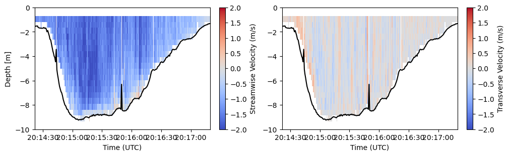
Next step is to calculate the water depth from one of the ADCP’s measurements. This can come from the bottom track ping, an altimeter ping, or an external depth sounder. You may need to do some quality control on this measurement, and make sure to add the range_offset, the depth of the ADCP below the waterline, to this array.
[6]:
# Find the water depth based on the average bottom track pings
water_depth = ds.attrs["range_offset"] + ds["dist_bt"].mean("beam").values
And we can superimpose that on our plot.
[7]:
fig, ax = plt.subplots(1,2, figsize=(10,3), constrained_layout=True)
s = ax[0].pcolormesh(ds["time"].values, -ds["range"].values, ds["vel"][0], cmap="coolwarm", vmin=-2, vmax=2)
t = ax[1].pcolormesh(ds["time"].values, -ds["range"].values, ds["vel"][1], cmap="coolwarm", vmin=-2, vmax=2)
ax[0].plot(ds["time"].values, -water_depth, color="k", label="Water Depth")
ax[1].plot(ds["time"].values, -water_depth, color="k", label="Water Depth")
fig.colorbar(s, ax=ax[0], label="Streamwise Velocity (m/s)")
fig.colorbar(t, ax=ax[1], label="Transverse Velocity (m/s)")
for a in ax:
    a.set(xlabel="Time (UTC)", ylim=(-10, 0))
ax[0].set(ylabel="Depth [m]")
[7]:
[Text(0, 0.5, 'Depth [m]')]
Now we can use the discharge function to calculate discharge, among other values (including power [W], power density [W/m^2], and the channel’s Reynolds Number). This function does quite a number of things internally: 1. Linearly extrapolates velocity to the riverbed/seafloor (assumes velocity at the seafloor, specified by the “water_depth” input, is 0 m/s) 2. Constant extrapolation of velocity to the water surface (water velocity at the uppermost bin is the same speed as that at the water
surface) 3. Remaps the velocity transect from “time” onto “distance” based on the GPS-measured location (latitude_gps and longitude_gps variables). It does this by converting the lat/lon to UTM and interpolating the UTM location onto the timegrid. 4. Velocity data is then integrated over the cross-sectional area to find discharge [m^3/s], power [W], power density [W/m^2], and hydraulic depth [m]. The last is used to find the Reynolds Number. 5. Values are saved into the returned dataset
The inputs are as follows: 1. ds - ADCP dataset 2. water_depth - as calculated above 3. rho - water density for the water current in question 4. mu - kinematic viscosity, based on the water temperature and salinity. Can be found from a look-up table online. 5. surface_offset - Location of water surface on a vertical datum. Typically will be 0 for a river. In a tidal channel, this will depend on the height of the tide relative to MLLW (or MSL or desired level) at the time of
the transect measurement. If the water level during the transect is above MLLW, this value will be negative. If above MLLW, this value will be positive. 6. utm_zone - UTM zone at the survey location. Can easily be found for a specific location by searching here: https://www.usgs.gov/media/images/mapping-utm-grid-conterminous-48-united-states
[8]:
# Calculate discharge, power, power density, and the Reynolds number of the channel
dolfyn.adp.api.discharge(ds, water_depth, rho=1020, mu=0.0012, surface_offset=0, utm_zone=5)
[8]:
<xarray.Dataset> Size: 236kB
Dimensions:              (time: 262, time_gps: 262, range: 24, range_sl: 5,
                          beam: 4, dir: 4, x1: 4, x2: 4, earth: 3, inst: 3)
Coordinates:
  * time                 (time) datetime64[ns] 2kB 2022-08-19T20:14:21.930000...
  * time_gps             (time_gps) datetime64[ns] 2kB 2022-08-19T20:14:23.59...
  * range                (range) float32 96B 0.95 1.43 1.91 ... 11.51 11.99
  * range_sl             (range_sl) float64 40B 0.54 0.66 0.78 0.9 1.02
  * beam                 (beam) int32 16B 1 2 3 4
  * dir                  (dir) <U10 160B 'streamwise' 'x-stream' 'vert' 'err'
  * x1                   (x1) int32 16B 1 2 3 4
  * x2                   (x2) int32 16B 1 2 3 4
  * earth                (earth) <U1 12B 'E' 'N' 'U'
  * inst                 (inst) <U1 12B 'X' 'Y' 'Z'
Data variables: (12/47)
    number               (time) uint32 1kB 398 399 400 401 ... 656 657 658 659
    builtin_test_fail    (time) bool 262B False False False ... False False
    c_sound              (time) float32 1kB 1.458e+03 1.458e+03 ... 1.459e+03
    depth                (time) float32 1kB 0.0 0.0 0.0 0.0 ... 0.0 0.0 0.0 0.0
    pitch                (time) float32 1kB -1.21 -1.01 -1.46 ... -0.5 -0.57
    roll                 (time) float32 1kB 1.97 0.49 1.07 ... -0.66 -0.53 0.72
    ...                   ...
    beam2inst_orientmat  (x1, x2) float32 64B 1.462 -1.462 0.0 ... -1.034 -1.034
    orientmat            (earth, inst, time) float32 9kB -0.8992 ... 0.9999
    discharge            float32 4B -1.136e+03
    power                float32 4B -1.211e+06
    power_density        float32 4B -1.307e+03
    reynolds_number      float32 4B 6.2e+06
Attributes: (12/46)
    prog_ver:                  56.1
    inst_make:                 TRDI
    inst_type:                 ADCP
    rotate_vars:               ['vel', 'vel_sl', 'vel_bt']
    has_imu:                   0
    inst_model:                RiverPro
    ...                        ...
    range_offset:              0.37
    blank_dist_sl:             0.05
    fs:                        1.47
    declination:               18
    declination_in_orientmat:  1
principal_heading: 173.522- time: 262
- time_gps: 262
- range: 24
- range_sl: 5
- beam: 4
- dir: 4
- x1: 4
- x2: 4
- earth: 3
- inst: 3
- time(time)datetime64[ns]2022-08-19T20:14:21.930000066 .....
- units :
- seconds since 1970-01-01 00:00:00
- long_name :
- Time
- standard_name :
- time
- coverage_content_type :
- coordinate
array(['2022-08-19T20:14:21.930000066', '2022-08-19T20:14:22.500000000', '2022-08-19T20:14:23.220000028', ..., '2022-08-19T20:17:18.329999923', '2022-08-19T20:17:18.910000085', '2022-08-19T20:17:19.450000047'], dtype='datetime64[ns]') - time_gps(time_gps)datetime64[ns]2022-08-19T20:14:23.599999904 .....
- units :
- seconds since 1970-01-01 00:00:00
- long_name :
- Time
- standard_name :
- time
- coverage_content_type :
- coordinate
array(['2022-08-19T20:14:23.599999904', '2022-08-19T20:14:24.200000047', '2022-08-19T20:14:25.000000000', ..., '2022-08-19T20:17:20.000000000', '2022-08-19T20:17:20.400000095', '2022-08-19T20:17:21.000000000'], dtype='datetime64[ns]') - range(range)float320.95 1.43 1.91 ... 11.51 11.99
- coverage_content_type :
- coordinate
- units :
- m
- long_name :
- Profile Range
- description :
- Distance to the center of each depth bin
array([ 0.95, 1.43, 1.91, 2.39, 2.87, 3.35, 3.83, 4.31, 4.79, 5.27, 5.75, 6.23, 6.71, 7.19, 7.67, 8.15, 8.63, 9.11, 9.59, 10.07, 10.55, 11.03, 11.51, 11.99], dtype=float32) - range_sl(range_sl)float640.54 0.66 0.78 0.9 1.02
- coverage_content_type :
- coordinate
- units :
- m
- long_name :
- Profile Range
- description :
- Distance to the center of each depth bin
array([0.54, 0.66, 0.78, 0.9 , 1.02])
- beam(beam)int321 2 3 4
- units :
- 1
- long_name :
- Beam Reference Frame
- coverage_content_type :
- coordinate
array([1, 2, 3, 4])
- dir(dir)<U10'streamwise' 'x-stream' ... 'err'
- units :
- 1
- long_name :
- Reference Frame
- coverage_content_type :
- coordinate
- ref_frame :
- principal
array(['streamwise', 'x-stream', 'vert', 'err'], dtype='<U10')
- x1(x1)int321 2 3 4
array([1, 2, 3, 4])
- x2(x2)int321 2 3 4
array([1, 2, 3, 4])
- earth(earth)<U1'E' 'N' 'U'
- units :
- 1
- long_name :
- Earth Reference Frame
- coverage_content_type :
- coordinate
array(['E', 'N', 'U'], dtype='<U1')
- inst(inst)<U1'X' 'Y' 'Z'
- units :
- 1
- long_name :
- Instrument Reference Frame
- coverage_content_type :
- coordinate
array(['X', 'Y', 'Z'], dtype='<U1')
- number(time)uint32398 399 400 401 ... 656 657 658 659
- units :
- 1
- long_name :
- Ensemble Number
- standard_name :
- number_of_observations
array([398, 399, 400, 401, 402, 403, 404, 405, 406, 407, 408, 409, 410, 411, 412, 413, 414, 415, 416, 417, 418, 419, 420, 421, 422, 423, 424, 425, 426, 427, 428, 429, 430, 431, 432, 433, 434, 435, 436, 437, 438, 439, 440, 441, 442, 443, 444, 445, 446, 447, 448, 449, 450, 451, 452, 453, 454, 455, 456, 457, 458, 459, 460, 461, 462, 463, 464, 465, 466, 467, 468, 469, 470, 471, 472, 473, 474, 475, 476, 477, 478, 479, 480, 481, 482, 483, 484, 485, 486, 487, 488, 489, 490, 491, 492, 493, 494, 495, 496, 497, 498, 499, 500, 501, 502, 503, 504, 505, 506, 507, 508, 509, 510, 511, 512, 513, 514, 515, 516, 517, 518, 519, 520, 521, 522, 523, 524, 525, 526, 527, 528, 529, 530, 531, 532, 533, 534, 535, 536, 537, 538, 539, 540, 541, 542, 543, 544, 545, 546, 547, 548, 549, 550, 551, 552, 553, 554, 555, 556, 557, 558, 559, 560, 561, 562, 563, 564, 565, 566, 567, 568, 569, 570, 571, 572, 573, 574, 575, 576, 577, 578, 579, 580, 581, 582, 583, 584, 585, 586, 587, 588, 589, 590, 591, 592, 593, 594, 595, 596, 597, 598, 599, 600, 601, 602, 603, 604, 605, 606, 607, 608, 609, 610, 611, 612, 613, 614, 615, 616, 617, 618, 619, 620, 621, 622, 623, 624, 625, 626, 627, 628, 629, 630, 631, 632, 633, 634, 635, 636, 637, 638, 639, 640, 641, 642, 643, 644, 645, 646, 647, 648, 649, 650, 651, 652, 653, 654, 655, 656, 657, 658, 659], dtype=uint32) - builtin_test_fail(time)boolFalse False False ... False False
- units :
- 1
- long_name :
- Built-In Test Failures
array([False, False, False, False, False, False, False, False, False, False, False, False, False, False, False, False, False, False, False, False, False, False, False, False, False, False, False, False, False, False, False, False, False, False, False, False, False, False, False, False, False, False, False, False, False, False, False, False, False, False, False, False, False, False, False, False, False, False, False, False, False, False, False, False, False, False, False, False, False, False, False, False, False, False, False, False, False, False, False, False, False, False, False, False, False, False, False, False, False, False, False, False, False, False, False, False, False, False, False, False, False, False, False, False, False, False, False, False, False, False, False, False, False, False, False, False, False, False, False, False, False, False, False, False, False, False, False, False, False, False, False, False, False, False, False, False, False, False, False, False, False, False, False, False, False, False, False, False, False, False, False, False, False, False, False, False, False, False, False, False, False, False, False, False, False, False, False, False, False, False, False, False, False, False, False, False, False, False, False, False, False, False, False, False, False, False, False, False, False, False, False, False, False, False, False, False, False, False, False, False, False, False, False, False, False, False, False, False, False, False, False, False, False, False, False, False, False, False, False, False, False, False, False, False, False, False, False, False, False, False, False, False, False, False, False, False, False, False, False, False, False, False, False, False, False, False, False, False, False, False, False, False, False, False, False, False, False, False, False, False, False, False]) - c_sound(time)float321.458e+03 1.458e+03 ... 1.459e+03
- units :
- m s-1
- long_name :
- Speed of Sound
- standard_name :
- speed_of_sound_in_sea_water
array([1458., 1458., 1458., 1458., 1458., 1458., 1458., 1458., 1458., 1458., 1458., 1458., 1458., 1458., 1458., 1458., 1458., 1458., 1458., 1458., 1458., 1458., 1458., 1458., 1458., 1458., 1458., 1458., 1458., 1458., 1458., 1458., 1458., 1458., 1458., 1458., 1458., 1458., 1458., 1458., 1458., 1458., 1458., 1458., 1458., 1458., 1458., 1458., 1458., 1458., 1458., 1458., 1458., 1458., 1458., 1458., 1458., 1458., 1458., 1458., 1458., 1458., 1458., 1458., 1458., 1458., 1458., 1458., 1458., 1458., 1458., 1458., 1458., 1458., 1458., 1458., 1458., 1458., 1458., 1458., 1458., 1458., 1458., 1458., 1458., 1458., 1458., 1458., 1458., 1458., 1458., 1458., 1458., 1458., 1458., 1458., 1458., 1458., 1458., 1458., 1458., 1458., 1458., 1458., 1458., 1458., 1458., 1458., 1458., 1458., 1458., 1458., 1458., 1458., 1458., 1458., 1458., 1458., 1458., 1458., 1458., 1458., 1458., 1458., 1458., 1458., 1458., 1458., 1458., 1458., 1458., 1458., 1458., 1458., 1458., 1458., 1459., 1459., 1458., 1458., 1458., 1458., 1458., 1458., 1458., 1458., 1458., 1458., 1458., 1458., 1458., 1458., 1458., 1458., 1458., 1458., 1458., 1458., 1458., 1458., 1458., 1458., 1458., 1458., 1458., 1458., 1458., 1459., 1458., 1458., 1458., 1458., 1458., 1458., 1458., 1458., 1458., 1458., 1458., 1458., 1458., 1458., 1458., 1458., 1458., 1458., 1458., 1458., 1458., 1458., 1458., 1458., 1458., 1458., 1458., 1458., 1458., 1458., 1458., 1458., 1458., 1458., 1458., 1458., 1458., 1458., 1458., 1458., 1458., 1458., 1458., 1458., 1458., 1458., 1458., 1458., 1458., 1458., 1458., 1458., 1458., 1458., 1458., 1458., 1458., 1458., 1458., 1458., 1458., 1458., 1459., 1459., 1458., 1458., 1459., 1459., 1459., 1459., 1459., 1458., 1458., 1458., 1458., 1459., 1459., 1458., 1458., 1459., 1459., 1459., 1459., 1459., 1459., 1459., 1459., 1459., 1459., 1459., 1459., 1459., 1459., 1459.], dtype=float32) - depth(time)float320.0 0.0 0.0 0.0 ... 0.0 0.0 0.0 0.0
- units :
- m
- long_name :
- Depth
- standard_name :
- depth
array([0., 0., 0., 0., 0., 0., 0., 0., 0., 0., 0., 0., 0., 0., 0., 0., 0., 0., 0., 0., 0., 0., 0., 0., 0., 0., 0., 0., 0., 0., 0., 0., 0., 0., 0., 0., 0., 0., 0., 0., 0., 0., 0., 0., 0., 0., 0., 0., 0., 0., 0., 0., 0., 0., 0., 0., 0., 0., 0., 0., 0., 0., 0., 0., 0., 0., 0., 0., 0., 0., 0., 0., 0., 0., 0., 0., 0., 0., 0., 0., 0., 0., 0., 0., 0., 0., 0., 0., 0., 0., 0., 0., 0., 0., 0., 0., 0., 0., 0., 0., 0., 0., 0., 0., 0., 0., 0., 0., 0., 0., 0., 0., 0., 0., 0., 0., 0., 0., 0., 0., 0., 0., 0., 0., 0., 0., 0., 0., 0., 0., 0., 0., 0., 0., 0., 0., 0., 0., 0., 0., 0., 0., 0., 0., 0., 0., 0., 0., 0., 0., 0., 0., 0., 0., 0., 0., 0., 0., 0., 0., 0., 0., 0., 0., 0., 0., 0., 0., 0., 0., 0., 0., 0., 0., 0., 0., 0., 0., 0., 0., 0., 0., 0., 0., 0., 0., 0., 0., 0., 0., 0., 0., 0., 0., 0., 0., 0., 0., 0., 0., 0., 0., 0., 0., 0., 0., 0., 0., 0., 0., 0., 0., 0., 0., 0., 0., 0., 0., 0., 0., 0., 0., 0., 0., 0., 0., 0., 0., 0., 0., 0., 0., 0., 0., 0., 0., 0., 0., 0., 0., 0., 0., 0., 0., 0., 0., 0., 0., 0., 0., 0., 0., 0., 0., 0., 0., 0., 0., 0., 0., 0., 0.], dtype=float32) - pitch(time)float32-1.21 -1.01 -1.46 ... -0.5 -0.57
- units :
- degree
- long_name :
- Pitch
- standard_name :
- platform_pitch
array([-1.21, -1.01, -1.46, -1.61, -0.25, -0.25, -0.25, -0.58, -1.57, -1.61, -2.01, -0.44, 0.07, -0.82, -0.69, -1.4 , -1.49, -1.01, -1.23, -1.38, -0.82, -0.18, -0.7 , -0.83, -0.71, -1.47, -0.36, -1.58, -2.57, -2.37, -0.7 , -0.37, -1.31, -0.64, 0.33, -1.54, 0.13, -0.37, -0.81, 0.26, -1.96, -0.44, -2.18, -0.12, -0.89, -1.16, -0.12, 0.14, 0.97, -0.69, 0.01, -1.99, -0.69, -2.12, 0.52, 0.33, -0.32, 0.46, 0.33, 0.33, 0.33, 0.33, 0.52, 0.39, 0.14, -1.09, -2.62, -0.37, -2.54, -0.78, -0.94, -1.14, -0.99, -0.99, -0.56, -0.56, -0.56, -1.89, -0.82, -2.95, 0.08, -1.82, -3.25, -1.65, -2.7 , -0.56, -0.84, 0.52, -0.45, -1.99, -0.43, -1.03, 0.46, -0.95, -0.58, -0.89, -0.7 , 0. , 0.78, -1.93, -1.41, -1.83, -0.5 , 0.78, -0.87, 0.53, 1.04, 0.2 , -0.19, -0.46, -2.8 , -0.31, -1.86, 0.07, 1.1 , -1.01, 0.14, 1.23, 0.2 , -1.14, 0.26, -0.95, 1.68, -4. , -0.98, -0.57, -1.78, -3.35, 0.21, 0.39, -0.69, -0.88, -1.93, 0.33, -0.51, -3.12, -1.93, -0.13, -0.44, 0.84, -0.44, 0.39, 0.71, 0.4 , 1.09, 0.65, 1.99, -0.37, 1.93, 1.03, 2.13, 2.13, 2.13, -0.7 , -0.05, -0.05, -0.05, 0.72, -1.19, 0.2 , 0.46, -2. , -0.37, -2.08, 1.29, 0.59, -1.08, 0.14, -1.01, -2.67, -0.58, 0.08, 0.4 , 1.93, 0.14, 1.86, -1.73, -3.07, 0.39, 0.39, -1.19, -0.31, -2.44, -0.63, -0.57, -1.16, -1.32, -1.87, -2.41, -0.57, -2.4 , -1.44, -1.74, -1.2 , 0.91, -1.29, -1.74, 0.65, 1.36, -1.96, 0.01, -0.31, -1.79, -0.37, 0.2 , -1.98, 0.14, 0.08, 0.39, -1.51, 1.17, -0.26, -0.18, -0.18, -0.18, -0.12, -0.19, 0.14, -1.08, -0.06, -2.2 , -2.2 , -2.2 , 0.52, -1.17, -0.62, -0.44, -0.76, -1.78, -0.87, -1.26, -1.01, -0.44, -0.77, -0.44, -0.44, -1.23, -0.31, 0.21, -0.19, -0.88, -0.64, -0.32, -1.2 , -1.77, -0.88, 0.27, 0.71, -0.25, -0.3 , -0.5 , -0.13, -1.13, -0.37, -0.12, 0.07, -0.96, -1.41, -1.46, -0.19, -0.5 , -0.57], dtype=float32) - roll(time)float321.97 0.49 1.07 ... -0.66 -0.53 0.72
- units :
- degree
- long_name :
- Roll
- standard_name :
- platform_roll
array([ 1.97, 0.49, 1.07, 1.05, 0.01, 0.01, 0.01, -0.47, 2.04, -0.46, 0.97, -0.21, 0.18, -0.43, -0.43, 1.62, 1.74, 0.24, 0.6 , 1.44, -0.15, 0.88, 0.66, 0.31, -1.3 , 2. , 1.14, 1.61, 1.65, 1.66, 1.01, 1.35, 1.53, 0.3 , 0.11, 1.44, 0.63, 0.42, 1.37, 0.37, 0.24, -0.05, -0.49, 0.62, -0.5 , 0.28, 1.61, 0.01, 0.8 , 1.32, 1.67, 1.98, 1.67, 0.05, -0.31, 0.59, -1.75, -0.47, -0.05, -0.05, -0.05, 2.34, 1.18, 0.14, 1.73, 0.95, -0.65, -0.63, 0.32, 0.41, 1.32, 0.72, 0.13, 0.52, 1.79, 1.79, 1.79, 1.06, 0.98, 1.7 , 1.87, 0.19, 0.39, 0.69, -1. , 2.83, 2.61, 1.54, 1.96, 2.17, 0.77, 1.8 , 0.58, 0.33, 0.6 , 0.85, 0.37, 0.11, 1.35, 0.76, 1.08, 0.58, 1.14, -0.86, 0.93, 2.13, 1.92, 2.16, 1.66, -1.76, 2.93, -0.08, -0.43, -0.53, -0.83, 2.42, 0.69, 2.91, 0.99, 1.33, -0.88, 0.27, 3.6 , 1.87, -1.18, 0.47, 0.95, 0.96, 2.87, 2.13, 2.13, 0.87, 0.6 , -1.4 , -2.45, 0.23, 0.02, -0.24, 1.62, 1.12, 1.16, -0.79, 0.79, 4.73, -0.76, -0.98, 0.63, 1.22, -0.41, 0.07, -2.18, -2.18, -2.18, -0.34, 0.94, 0.94, 0.94, 1.06, 1.05, -0.37, 0.32, 1.44, 1.31, 0.36, 1.08, 1.06, 1.96, -0.44, -0.18, 1.65, 0.57, 1.18, 1.12, -0.51, -0.41, -3.35, -1.45, 0.18, -0.57, -0.76, 1.86, 1.27, -0.62, 0.39, 1.01, 1.7 , 0.55, -0.46, 0.66, -1.07, 1.1 , 0.29, 2.38, 0.36, -0.34, -0.11, 1.09, 1.17, 1.58, 0.22, -0.69, 0.17, 1.63, -0.28, 0.2 , 1.65, 1.9 , 2.5 , -0.66, 0.2 , -0.25, -0.43, 0.2 , 0.2 , 0.2 , -2.13, -0.02, -1.2 , -0.37, -0.21, 0.87, 0.87, 0.87, 0.59, 0.9 , 0.7 , 0.01, 2.11, 1.01, -0.09, 0.92, 0.97, 1.42, 1.56, 0.4 , 0.37, -0.53, -0.28, 0.57, 1.08, 0.55, 0.43, 0.53, 0.2 , 0.43, 1.64, 0.23, -0.41, 0.56, 0.84, 0.72, -0.27, 1.38, 0.72, -0.24, -0.18, 1.21, 0.76, 1.3 , -0.66, -0.53, 0.72], dtype=float32) - heading(time)float32-154.2 -146.9 ... 159.4 155.4
- units :
- degree
- long_name :
- Heading
- standard_name :
- platform_orientation
array([-154.16, -146.94, -149.73, -149.08, -142.38, -142.38, -142.38, -138.54, -150.82, -140.2 , -145.69, -138.74, -138.54, -137.62, -137.32, -146.94, -147.46, -141.54, -145.16, -150.39, -147.23, -152.72, -155.97, -157.79, -153.27, -170.08, -169.21, -172.79, -173.52, -174.86, -174.83, -178.64, -177.88, -174.07, -174.06, -178.08, -177.42, -175.4 , -179.11, -176.44, -172.87, -174.05, -170.72, -178.3 , -172.07, -175.75, 176.65, -176.27, 178.85, 178.7 , 175.97, 178.48, 177.12, -175.92, -177.85, 177.34, -171.18, -178.37, 179.31, 179.31, 179.31, 167.96, 172.52, 177.7 , 170.57, 175.68, -176.88, 178.71, 178.44, 174.43, 171.22, 173.2 , 175.78, 174.36, 169.04, 169.04, 169.04, 174.78, 173.5 , 174.49, 167.44, 175.53, 175.54, 170.25, 177.2 , 157.25, 157.76, 157.99, 158.78, 161.56, 161.43, 158.78, 159.33, 163.81, 163.14, 163.47, 166.03, 166.89, 160.38, 169.02, 166.81, 170.04, 165.43, 169.3 , 166.31, 159.1 , 158.09, 159.45, 162.64, 176.71, 164.01, 168.79, 173.7 , 170.36, 169.52, 162.49, 165.44, 154.91, 164.57, 166.59, 171.5 , 169.89, 152.04, 171.17, -179.85, 171.93, 170.65, 173.46, 159.55, 161.73, 163.4 , 167.76, 171.29, 174.45, -178.8 , 174.32, 173.31, 171.61, 165.1 , 164.11, 166.82, 173.13, 166.24, 154.54, 173.9 , 176.31, 165.78, 168.37, 170.27, 169.04, 176.61, 176.61, 176.61, 173.82, 166.56, 166.56, 166.56, 164.95, 168.67, 171.44, 166.63, 167.48, 163.93, 170.73, 159.4 , 161.15, 161.24, 165.7 , 165.39, 165.08, 163.16, 159.8 , 159.5 , 161.17, 166.81, 176.11, 173.99, 170.09, 163.81, 163.81, 158.22, 156.79, 167.65, 158.87, 156.31, 155.09, 158.19, 162.2 , 159.09, 159.77, 158.65, 159.81, 154. , 158.14, 154.61, 160.49, 158.01, 151.21, 147.92, 162.34, 160.3 , 157.92, 157.12, 160.22, 156.76, 157.91, 151.12, 149.55, 158.79, 161.03, 154.09, 160.07, 158.06, 158.06, 158.06, 166.28, 158.86, 162.37, 162.58, 159.29, 160.53, 160.53, 160.53, 151.05, 156.2 , 155.22, 156.83, 150.5 , 156.62, 157.63, 154.88, 154.28, 151.08, 150.79, 153.06, 153.4 , 157.91, 154.43, 150.07, 149.9 , 153.38, 152.86, 152.34, 156.03, 157.2 , 151.1 , 152.18, 152.47, 153.35, 152.24, 153.47, 156.04, 154.19, 154.04, 156.93, 156.44, 154.83, 157.14, 155.93, 158.46, 159.43, 155.37], dtype=float32) - temp(time)float3213.13 13.13 13.13 ... 13.19 13.25
- units :
- degree_C
- long_name :
- Temperature
- standard_name :
- sea_water_temperature
array([13.13, 13.13, 13.13, 13.13, 13.13, 13.13, 13.13, 13.13, 13.13, 13.13, 13.13, 13.13, 13.13, 13.13, 13.13, 13.13, 13.13, 13.13, 13.06, 13.06, 13.13, 13.13, 13.13, 13.13, 13.13, 13.13, 13.13, 13.13, 13.13, 13.13, 13.13, 13.13, 13.13, 13.13, 13.13, 13.13, 13.13, 13.13, 13.13, 13.13, 13.13, 13.13, 13.13, 13.13, 13.13, 13.13, 13.13, 13.13, 13.13, 13.13, 13.13, 13.13, 13.13, 13.13, 13.13, 13.13, 13.13, 13.13, 13.13, 13.13, 13.13, 13.13, 13.13, 13.13, 13.13, 13.13, 13.13, 13.13, 13.13, 13.13, 13.13, 13.13, 13.13, 13.13, 13.13, 13.13, 13.13, 13.13, 13.13, 13.13, 13.13, 13.13, 13.13, 13.13, 13.13, 13.13, 13.13, 13.13, 13.13, 13.13, 13.13, 13.13, 13.13, 13.13, 13.13, 13.13, 13.13, 13.13, 13.13, 13.13, 13.13, 13.13, 13.13, 13.13, 13.13, 13.13, 13.13, 13.13, 13.13, 13.13, 13.13, 13.13, 13.13, 13.13, 13.13, 13.13, 13.13, 13.13, 13.13, 13.13, 13.13, 13.13, 13.13, 13.13, 13.13, 13.13, 13.13, 13.13, 13.13, 13.13, 13.13, 13.13, 13.13, 13.13, 13.13, 13.13, 13.19, 13.19, 13.13, 13.13, 13.13, 13.13, 13.13, 13.13, 13.13, 13.13, 13.13, 13.13, 13.13, 13.13, 13.13, 13.13, 13.13, 13.13, 13.13, 13.13, 13.13, 13.13, 13.13, 13.13, 13.13, 13.13, 13.13, 13.13, 13.13, 13.13, 13.13, 13.19, 13.13, 13.13, 13.13, 13.13, 13.13, 13.13, 13.13, 13.13, 13.13, 13.13, 13.13, 13.13, 13.13, 13.13, 13.13, 13.13, 13.13, 13.13, 13.13, 13.13, 13.13, 13.13, 13.13, 13.13, 13.13, 13.13, 13.13, 13.13, 13.13, 13.13, 13.13, 13.13, 13.13, 13.13, 13.13, 13.13, 13.13, 13.13, 13.13, 13.13, 13.13, 13.13, 13.13, 13.13, 13.13, 13.13, 13.13, 13.13, 13.13, 13.13, 13.13, 13.13, 13.13, 13.13, 13.13, 13.13, 13.13, 13.13, 13.13, 13.13, 13.13, 13.13, 13.19, 13.19, 13.13, 13.13, 13.19, 13.19, 13.19, 13.19, 13.19, 13.13, 13.13, 13.13, 13.13, 13.19, 13.19, 13.13, 13.13, 13.19, 13.19, 13.19, 13.19, 13.19, 13.19, 13.19, 13.19, 13.19, 13.19, 13.19, 13.19, 13.19, 13.19, 13.25], dtype=float32) - salinity(time)float320.0 0.0 0.0 0.0 ... 0.0 0.0 0.0 0.0
- units :
- psu
- long_name :
- Salinity
- standard_name :
- sea_water_salinity
array([0., 0., 0., 0., 0., 0., 0., 0., 0., 0., 0., 0., 0., 0., 0., 0., 0., 0., 0., 0., 0., 0., 0., 0., 0., 0., 0., 0., 0., 0., 0., 0., 0., 0., 0., 0., 0., 0., 0., 0., 0., 0., 0., 0., 0., 0., 0., 0., 0., 0., 0., 0., 0., 0., 0., 0., 0., 0., 0., 0., 0., 0., 0., 0., 0., 0., 0., 0., 0., 0., 0., 0., 0., 0., 0., 0., 0., 0., 0., 0., 0., 0., 0., 0., 0., 0., 0., 0., 0., 0., 0., 0., 0., 0., 0., 0., 0., 0., 0., 0., 0., 0., 0., 0., 0., 0., 0., 0., 0., 0., 0., 0., 0., 0., 0., 0., 0., 0., 0., 0., 0., 0., 0., 0., 0., 0., 0., 0., 0., 0., 0., 0., 0., 0., 0., 0., 0., 0., 0., 0., 0., 0., 0., 0., 0., 0., 0., 0., 0., 0., 0., 0., 0., 0., 0., 0., 0., 0., 0., 0., 0., 0., 0., 0., 0., 0., 0., 0., 0., 0., 0., 0., 0., 0., 0., 0., 0., 0., 0., 0., 0., 0., 0., 0., 0., 0., 0., 0., 0., 0., 0., 0., 0., 0., 0., 0., 0., 0., 0., 0., 0., 0., 0., 0., 0., 0., 0., 0., 0., 0., 0., 0., 0., 0., 0., 0., 0., 0., 0., 0., 0., 0., 0., 0., 0., 0., 0., 0., 0., 0., 0., 0., 0., 0., 0., 0., 0., 0., 0., 0., 0., 0., 0., 0., 0., 0., 0., 0., 0., 0., 0., 0., 0., 0., 0., 0., 0., 0., 0., 0., 0., 0.], dtype=float32) - min_preping_wait(time)float32420.8 420.4 420.1 ... 600.7 600.3
- units :
- s
- long_name :
- Minimum Pre-Ping Wait Time Between Measurements
array([420.78, 420.39, 420.07, 420.79, 420.46, 420.37, 420.05, 420.71, 420.43, 420.1 , 420.81, 420.49, 420.22, 420.91, 420.53, 420.1 , 420.71, 420.37, 420.09, 420.81, 420.61, 420.3 , 420.1 , 420.9 , 420.56, 420.3 , 420.97, 420.66, 420.32, 420.03, 420.72, 420.46, 420.08, 420.76, 420.42, 420.13, 420.81, 420.55, 420.26, 420.01, 420.78, 420.57, 420.38, 420.22, 420.06, 420.66, 420.3 , 420.9 , 420.54, 420.14, 420.8 , 420.41, 420.09, 420.73, 420.42, 420.06, 420.76, 420.44, 420.15, 420.02, 420.71, 420.38, 420.08, 420.75, 420.46, 420.13, 420.85, 420.54, 420.27, 420.95, 420.68, 420.36, 420.08, 420.77, 420.5 , 420.36, 480.05, 480.72, 480.44, 480.11, 480.84, 480.51, 480.22, 480.88, 480.6 , 480.27, 480.98, 480.64, 480.36, 480.02, 480.72, 480.39, 480.1 , 480.77, 480.48, 480.13, 480.83, 480.49, 480.19, 480.85, 480.55, 480.21, 480.91, 480.57, 480.28, 480.94, 480.64, 480.31, 480. , 480.67, 480.38, 480.04, 480.75, 480.42, 480.12, 480.8 , 480.5 , 480.14, 480.83, 480.47, 480.15, 480.79, 480.48, 480.11, 480.76, 480.39, 480.05, 480.68, 480.34, 480.99, 480.67, 480.32, 480.01, 480.65, 480.34, 480.98, 480.66, 480.31, 480.99, 480.63, 480.29, 480.9 , 480.56, 480.17, 480.81, 480.41, 480.05, 480.66, 480.31, 480.91, 480.56, 480.36, 480.99, 480.6 , 480.26, 480.06, 480.69, 480.31, 480.94, 480.53, 480.16, 480.75, 480.39, 480.96, 480.78, 480.58, 540.39, 540.19, 540.98, 540.76, 540.48, 540.24, 540.95, 540.69, 540.39, 540.12, 540.8 , 540.54, 540.22, 540.96, 540.63, 540.36, 540.03, 540.73, 540.39, 540.09, 540.74, 540.43, 540.08, 540.78, 540.44, 540.14, 540.8 , 540.49, 540.13, 540.81, 540.45, 540.12, 540.74, 540.41, 540.02, 540.69, 540.3 , 540.94, 540.54, 540.28, 540.96, 540.69, 540.39, 540.13, 540.73, 540.46, 540.13, 540.02, 540.7 , 540.35, 540.02, 540.63, 540.29, 540.9 , 540.58, 540.4 , 540.04, 540.67, 540.34, 540.95, 540.61, 540.23, 540.95, 540.57, 540.36, 540.08, 540.84, 540.62, 540.4 , 540.17, 540.88, 540.64, 540.34, 540.09, 540.77, 540.43, 540.04, 540.7 , 540.32, 540.97, 540.57, 540.2 , 540.78, 540.41, 540.98, 540.59, 540.14, 540.75, 600.32, 600.92, 600.47, 600.07, 600.62, 600.21, 600.74, 600.33], dtype=float32) - heading_std(time)float320.0 0.0 0.0 0.0 ... 0.0 0.0 0.0 0.0
- units :
- degree
- long_name :
- Heading Standard Deviation
array([0., 0., 0., 0., 0., 0., 0., 0., 0., 0., 0., 0., 0., 0., 0., 0., 0., 0., 0., 0., 0., 0., 0., 0., 0., 0., 0., 0., 0., 0., 0., 0., 0., 0., 0., 0., 0., 0., 0., 0., 0., 0., 0., 0., 0., 0., 0., 0., 0., 0., 0., 0., 0., 0., 0., 0., 0., 0., 0., 0., 0., 0., 0., 0., 0., 0., 0., 0., 0., 0., 0., 0., 0., 0., 0., 0., 0., 0., 0., 0., 0., 0., 0., 0., 0., 0., 0., 0., 0., 0., 0., 0., 0., 0., 0., 0., 0., 0., 0., 0., 0., 0., 0., 0., 0., 0., 0., 0., 0., 0., 0., 0., 0., 0., 0., 0., 0., 0., 0., 0., 0., 0., 0., 0., 0., 0., 0., 0., 0., 0., 0., 0., 0., 0., 0., 0., 0., 0., 0., 0., 0., 0., 0., 0., 0., 0., 0., 0., 0., 0., 0., 0., 0., 0., 0., 0., 0., 0., 0., 0., 0., 0., 0., 0., 0., 0., 0., 0., 0., 0., 0., 0., 0., 0., 0., 0., 0., 0., 0., 0., 0., 0., 0., 0., 0., 0., 0., 0., 0., 0., 0., 0., 0., 0., 0., 0., 0., 0., 0., 0., 0., 0., 0., 0., 0., 0., 0., 0., 0., 0., 0., 0., 0., 0., 0., 0., 0., 0., 0., 0., 0., 0., 0., 0., 0., 0., 0., 0., 0., 0., 0., 0., 0., 0., 0., 0., 0., 0., 0., 0., 0., 0., 0., 0., 0., 0., 0., 0., 0., 0., 0., 0., 0., 0., 0., 0., 0., 0., 0., 0., 0., 0.], dtype=float32) - pitch_std(time)float320.0 0.0 0.0 0.0 ... 0.0 0.0 0.0 0.0
- units :
- degree
- long_name :
- Pitch Standard Deviation
array([0., 0., 0., 0., 0., 0., 0., 0., 0., 0., 0., 0., 0., 0., 0., 0., 0., 0., 0., 0., 0., 0., 0., 0., 0., 0., 0., 0., 0., 0., 0., 0., 0., 0., 0., 0., 0., 0., 0., 0., 0., 0., 0., 0., 0., 0., 0., 0., 0., 0., 0., 0., 0., 0., 0., 0., 0., 0., 0., 0., 0., 0., 0., 0., 0., 0., 0., 0., 0., 0., 0., 0., 0., 0., 0., 0., 0., 0., 0., 0., 0., 0., 0., 0., 0., 0., 0., 0., 0., 0., 0., 0., 0., 0., 0., 0., 0., 0., 0., 0., 0., 0., 0., 0., 0., 0., 0., 0., 0., 0., 0., 0., 0., 0., 0., 0., 0., 0., 0., 0., 0., 0., 0., 0., 0., 0., 0., 0., 0., 0., 0., 0., 0., 0., 0., 0., 0., 0., 0., 0., 0., 0., 0., 0., 0., 0., 0., 0., 0., 0., 0., 0., 0., 0., 0., 0., 0., 0., 0., 0., 0., 0., 0., 0., 0., 0., 0., 0., 0., 0., 0., 0., 0., 0., 0., 0., 0., 0., 0., 0., 0., 0., 0., 0., 0., 0., 0., 0., 0., 0., 0., 0., 0., 0., 0., 0., 0., 0., 0., 0., 0., 0., 0., 0., 0., 0., 0., 0., 0., 0., 0., 0., 0., 0., 0., 0., 0., 0., 0., 0., 0., 0., 0., 0., 0., 0., 0., 0., 0., 0., 0., 0., 0., 0., 0., 0., 0., 0., 0., 0., 0., 0., 0., 0., 0., 0., 0., 0., 0., 0., 0., 0., 0., 0., 0., 0., 0., 0., 0., 0., 0., 0.], dtype=float32) - roll_std(time)float320.0 0.0 0.0 0.0 ... 0.0 0.0 0.0 0.0
- units :
- degree
- long_name :
- Roll Standard Deviation
array([0., 0., 0., 0., 0., 0., 0., 0., 0., 0., 0., 0., 0., 0., 0., 0., 0., 0., 0., 0., 0., 0., 0., 0., 0., 0., 0., 0., 0., 0., 0., 0., 0., 0., 0., 0., 0., 0., 0., 0., 0., 0., 0., 0., 0., 0., 0., 0., 0., 0., 0., 0., 0., 0., 0., 0., 0., 0., 0., 0., 0., 0., 0., 0., 0., 0., 0., 0., 0., 0., 0., 0., 0., 0., 0., 0., 0., 0., 0., 0., 0., 0., 0., 0., 0., 0., 0., 0., 0., 0., 0., 0., 0., 0., 0., 0., 0., 0., 0., 0., 0., 0., 0., 0., 0., 0., 0., 0., 0., 0., 0., 0., 0., 0., 0., 0., 0., 0., 0., 0., 0., 0., 0., 0., 0., 0., 0., 0., 0., 0., 0., 0., 0., 0., 0., 0., 0., 0., 0., 0., 0., 0., 0., 0., 0., 0., 0., 0., 0., 0., 0., 0., 0., 0., 0., 0., 0., 0., 0., 0., 0., 0., 0., 0., 0., 0., 0., 0., 0., 0., 0., 0., 0., 0., 0., 0., 0., 0., 0., 0., 0., 0., 0., 0., 0., 0., 0., 0., 0., 0., 0., 0., 0., 0., 0., 0., 0., 0., 0., 0., 0., 0., 0., 0., 0., 0., 0., 0., 0., 0., 0., 0., 0., 0., 0., 0., 0., 0., 0., 0., 0., 0., 0., 0., 0., 0., 0., 0., 0., 0., 0., 0., 0., 0., 0., 0., 0., 0., 0., 0., 0., 0., 0., 0., 0., 0., 0., 0., 0., 0., 0., 0., 0., 0., 0., 0., 0., 0., 0., 0., 0., 0.], dtype=float32) - pressure(time)float320.0 0.0 0.0 0.0 ... 0.0 0.0 0.0 0.0
- units :
- dbar
- long_name :
- Pressure
- standard_name :
- sea_water_pressure
array([0., 0., 0., 0., 0., 0., 0., 0., 0., 0., 0., 0., 0., 0., 0., 0., 0., 0., 0., 0., 0., 0., 0., 0., 0., 0., 0., 0., 0., 0., 0., 0., 0., 0., 0., 0., 0., 0., 0., 0., 0., 0., 0., 0., 0., 0., 0., 0., 0., 0., 0., 0., 0., 0., 0., 0., 0., 0., 0., 0., 0., 0., 0., 0., 0., 0., 0., 0., 0., 0., 0., 0., 0., 0., 0., 0., 0., 0., 0., 0., 0., 0., 0., 0., 0., 0., 0., 0., 0., 0., 0., 0., 0., 0., 0., 0., 0., 0., 0., 0., 0., 0., 0., 0., 0., 0., 0., 0., 0., 0., 0., 0., 0., 0., 0., 0., 0., 0., 0., 0., 0., 0., 0., 0., 0., 0., 0., 0., 0., 0., 0., 0., 0., 0., 0., 0., 0., 0., 0., 0., 0., 0., 0., 0., 0., 0., 0., 0., 0., 0., 0., 0., 0., 0., 0., 0., 0., 0., 0., 0., 0., 0., 0., 0., 0., 0., 0., 0., 0., 0., 0., 0., 0., 0., 0., 0., 0., 0., 0., 0., 0., 0., 0., 0., 0., 0., 0., 0., 0., 0., 0., 0., 0., 0., 0., 0., 0., 0., 0., 0., 0., 0., 0., 0., 0., 0., 0., 0., 0., 0., 0., 0., 0., 0., 0., 0., 0., 0., 0., 0., 0., 0., 0., 0., 0., 0., 0., 0., 0., 0., 0., 0., 0., 0., 0., 0., 0., 0., 0., 0., 0., 0., 0., 0., 0., 0., 0., 0., 0., 0., 0., 0., 0., 0., 0., 0., 0., 0., 0., 0., 0., 0.], dtype=float32) - pressure_std(time)float320.0 0.0 0.0 0.0 ... 0.0 0.0 0.0 0.0
- units :
- dbar
- long_name :
- Pressure Standard Deviation
array([0., 0., 0., 0., 0., 0., 0., 0., 0., 0., 0., 0., 0., 0., 0., 0., 0., 0., 0., 0., 0., 0., 0., 0., 0., 0., 0., 0., 0., 0., 0., 0., 0., 0., 0., 0., 0., 0., 0., 0., 0., 0., 0., 0., 0., 0., 0., 0., 0., 0., 0., 0., 0., 0., 0., 0., 0., 0., 0., 0., 0., 0., 0., 0., 0., 0., 0., 0., 0., 0., 0., 0., 0., 0., 0., 0., 0., 0., 0., 0., 0., 0., 0., 0., 0., 0., 0., 0., 0., 0., 0., 0., 0., 0., 0., 0., 0., 0., 0., 0., 0., 0., 0., 0., 0., 0., 0., 0., 0., 0., 0., 0., 0., 0., 0., 0., 0., 0., 0., 0., 0., 0., 0., 0., 0., 0., 0., 0., 0., 0., 0., 0., 0., 0., 0., 0., 0., 0., 0., 0., 0., 0., 0., 0., 0., 0., 0., 0., 0., 0., 0., 0., 0., 0., 0., 0., 0., 0., 0., 0., 0., 0., 0., 0., 0., 0., 0., 0., 0., 0., 0., 0., 0., 0., 0., 0., 0., 0., 0., 0., 0., 0., 0., 0., 0., 0., 0., 0., 0., 0., 0., 0., 0., 0., 0., 0., 0., 0., 0., 0., 0., 0., 0., 0., 0., 0., 0., 0., 0., 0., 0., 0., 0., 0., 0., 0., 0., 0., 0., 0., 0., 0., 0., 0., 0., 0., 0., 0., 0., 0., 0., 0., 0., 0., 0., 0., 0., 0., 0., 0., 0., 0., 0., 0., 0., 0., 0., 0., 0., 0., 0., 0., 0., 0., 0., 0., 0., 0., 0., 0., 0., 0.], dtype=float32) - vel(dir, range, time)float32nan -1.378 -1.597 ... nan nan nan
- units :
- m s-1
- coverage_content_type :
- physicalMeasurement
- long_name :
- Water Velocity
array([[[ nan, -1.3780606e+00, -1.5968075e+00, ..., -2.6226619e-01, -2.5654507e-01, -2.2308642e-01], [ nan, -2.5692660e-01, -2.6959109e-01, ..., nan, nan, nan], [ nan, nan, nan, ..., nan, nan, nan], ..., [ nan, nan, nan, ..., nan, nan, nan], [ nan, nan, nan, ..., nan, nan, nan], [ nan, nan, nan, ..., nan, nan, nan]], [[ nan, 2.6142585e-01, -4.9651265e-03, ..., 3.5546001e-02, 3.3569042e-02, -1.2026111e-02], [ nan, 4.8740420e-02, -8.3826878e-04, ..., nan, nan, nan], [ nan, nan, nan, ..., nan, nan, nan], ... [ nan, nan, nan, ..., nan, nan, nan], [ nan, nan, nan, ..., nan, nan, nan], [ nan, nan, nan, ..., nan, nan, nan]], [[ nan, -3.6425743e-01, -7.1455896e-02, ..., 5.0781541e-02, -3.7472174e-03, 1.1241753e-02], [ nan, -6.7912415e-02, -1.2063992e-02, ..., nan, nan, nan], [ nan, nan, nan, ..., nan, nan, nan], ..., [ nan, nan, nan, ..., nan, nan, nan], [ nan, nan, nan, ..., nan, nan, nan], [ nan, nan, nan, ..., nan, nan, nan]]], dtype=float32) - amp(beam, range, time)uint8145 149 147 147 149 ... 0 0 0 0 0
- units :
- 1
- coverage_content_type :
- physicalMeasurement
- long_name :
- Acoustic Signal Amplitude
- standard_name :
- signal_intensity_from_multibeam_acoustic_doppler_velocity_sensor_in_sea_water
array([[[145, 149, 147, ..., 133, 131, 134], [138, 147, 148, ..., 85, 87, 86], [ 0, 0, 0, ..., 0, 0, 0], ..., [ 0, 0, 0, ..., 0, 0, 0], [ 0, 0, 0, ..., 0, 0, 0], [ 0, 0, 0, ..., 0, 0, 0]], [[145, 153, 151, ..., 137, 138, 136], [155, 164, 170, ..., 93, 90, 85], [ 0, 0, 0, ..., 0, 0, 0], ..., [ 0, 0, 0, ..., 0, 0, 0], [ 0, 0, 0, ..., 0, 0, 0], [ 0, 0, 0, ..., 0, 0, 0]], [[142, 145, 143, ..., 128, 128, 130], [154, 157, 155, ..., 85, 86, 87], [ 0, 0, 0, ..., 0, 0, 0], ..., [ 0, 0, 0, ..., 0, 0, 0], [ 0, 0, 0, ..., 0, 0, 0], [ 0, 0, 0, ..., 0, 0, 0]], [[141, 147, 147, ..., 135, 132, 132], [141, 139, 138, ..., 85, 88, 83], [ 0, 0, 0, ..., 0, 0, 0], ..., [ 0, 0, 0, ..., 0, 0, 0], [ 0, 0, 0, ..., 0, 0, 0], [ 0, 0, 0, ..., 0, 0, 0]]], dtype=uint8) - corr(beam, range, time)uint8135 113 114 107 117 ... 0 0 0 0 0
- units :
- 1
- coverage_content_type :
- physicalMeasurement
- long_name :
- Acoustic Signal Correlation
- standard_name :
- beam_consistency_indicator_from_multibeam_acoustic_doppler_velocity_profiler_in_sea_water
array([[[135, 113, 114, ..., 241, 245, 246], [110, 111, 115, ..., 136, 149, 145], [ 0, 0, 0, ..., 0, 0, 0], ..., [ 0, 0, 0, ..., 0, 0, 0], [ 0, 0, 0, ..., 0, 0, 0], [ 0, 0, 0, ..., 0, 0, 0]], [[173, 118, 110, ..., 240, 245, 247], [133, 110, 124, ..., 141, 143, 145], [ 0, 0, 0, ..., 0, 0, 0], ..., [ 0, 0, 0, ..., 0, 0, 0], [ 0, 0, 0, ..., 0, 0, 0], [ 0, 0, 0, ..., 0, 0, 0]], [[128, 114, 112, ..., 245, 244, 246], [134, 110, 109, ..., 138, 145, 148], [ 0, 0, 0, ..., 0, 0, 0], ..., [ 0, 0, 0, ..., 0, 0, 0], [ 0, 0, 0, ..., 0, 0, 0], [ 0, 0, 0, ..., 0, 0, 0]], [[151, 117, 118, ..., 241, 244, 246], [108, 101, 112, ..., 141, 150, 142], [ 0, 0, 0, ..., 0, 0, 0], ..., [ 0, 0, 0, ..., 0, 0, 0], [ 0, 0, 0, ..., 0, 0, 0], [ 0, 0, 0, ..., 0, 0, 0]]], dtype=uint8) - dist_bt(beam, time)float321.3 1.18 1.16 ... 1.04 0.96 0.96
- units :
- m
- coverage_content_type :
- physicalMeasurement
- long_name :
- Bottom Track Measured Depth
array([[1.3 , 1.18, 1.16, ..., 0.98, 0.96, 0.96], [1.11, 1.13, 1.09, ..., 0.97, 0.95, 0.97], [1.17, 1.12, 1.12, ..., 0.95, 0.97, 0.92], [1.24, 1.25, 1.26, ..., 1.04, 0.96, 0.96]], dtype=float32) - vel_bt(dir, time)float320.03986 0.02038 ... 0.007236
- units :
- m s-1
- coverage_content_type :
- physicalMeasurement
- long_name :
- Water Velocity
array([[ 0.03985795, 0.02037775, 0.03288013, ..., -0.01411782, -0.01381912, 0.04580029], [-0.07396869, -0.08312948, -0.07563345, ..., -0.6168041 , -0.6167893 , -0.5712449 ], [ 0.00555705, -0.00484052, -0.00232305, ..., 0.01484554, 0.0183713 , 0.00577757], [ 0.00413489, 0.00206744, -0.00103372, ..., 0.00206745, -0.00516861, 0.00723603]], dtype=float32) - corr_bt(beam, time)uint8251 251 253 249 ... 222 254 248 223
- units :
- 1
- coverage_content_type :
- physicalMeasurement
- long_name :
- Acoustic Signal Correlation
- standard_name :
- beam_consistency_indicator_from_multibeam_acoustic_doppler_velocity_profiler_in_sea_water
array([[251, 251, 253, ..., 234, 236, 231], [252, 251, 250, ..., 229, 252, 232], [249, 250, 243, ..., 224, 239, 228], [249, 252, 243, ..., 254, 248, 223]], dtype=uint8) - amp_bt(beam, time)uint835 31 29 33 39 ... 46 40 60 48 52
- units :
- 1
- coverage_content_type :
- physicalMeasurement
- long_name :
- Acoustic Signal Amplitude
- standard_name :
- signal_intensity_from_multibeam_acoustic_doppler_velocity_sensor_in_sea_water
array([[35, 31, 29, ..., 61, 74, 58], [36, 51, 54, ..., 47, 56, 52], [43, 56, 52, ..., 64, 51, 62], [42, 53, 48, ..., 60, 48, 52]], dtype=uint8) - prcnt_gd_bt(beam, time)uint80 0 0 0 0 0 0 0 ... 1 1 1 1 1 1 1 1
- units :
- %
- coverage_content_type :
- physicalMeasurement
- long_name :
- Percent Good
- standard_name :
- proportion_of_acceptable_signal_returns_from_acoustic_instrument_in_sea_water
array([[0, 0, 0, ..., 0, 0, 0], [0, 0, 0, ..., 0, 0, 0], [0, 0, 0, ..., 0, 0, 0], [1, 1, 1, ..., 1, 1, 1]], dtype=uint8) - alt_dist(time)float321.1 1.08 1.07 ... 1.02 0.98 0.97
- units :
- m
- long_name :
- Altimeter Range
- standard_name :
- altimeter_range
array([1.1 , 1.08 , 1.07 , 1.06 , 1.06 , 1.31 , 1.31 , 1.29 , 1.26 , 1.271, 1.22 , 1.21 , 1.21 , 1.13 , 1.22 , 1.21 , 1.23 , 1.37 , 1.45 , 1.46 , 1.4 , 1.64 , 2.03 , 2.217, 2.379, 2.52 , 2.75 , 2.99 , 3.54 , 3.58 , 3.83 , 4.179, 4.453, 4.52 , 4.729, 5.79 , 5.914, 5.966, 0. , 0. , 7.651, 7.394, 7.53 , 7.56 , 7.65 , 7.793, 7.893, 8.042, 8.172, 8.31 , 8.66 , 8.67 , 8.75 , 8.82 , 8.88 , 8.96 , 8.97 , 9.01 , 9.05 , 9.09 , 9.13 , 9.16 , 9.2 , 9.27 , 9.27 , 8.96 , 9.04 , 9.18 , 8.93 , 9.09 , 9.05 , 9.01 , 8.97 , 8.97 , 8.94 , 8.88 , 8.86 , 8.86 , 8.84 , 8.88 , 8.86 , 8.77 , 8.78 , 8.78 , 8.78 , 8.59 , 8.77 , 8.73 , 8.69 , 8.71 , 8.77 , 8.78 , 8.698, 8.698, 8.73 , 8.67 , 8.61 , 8.63 , 8.67 , 8.69 , 8.65 , 8.641, 8.61 , 8.584, 8.617, 8.698, 8.811, 8.887, 8.96 , 8.99 , 8.925, 9.01 , 8.754, 8.78 , 8.071, 8.635, 8.565, 8.4 , 8.35 , 8.27 , 7.58 , 8.142, 8.15 , 7.46 , 8.07 , 8.136, 8.243, 8.261, 7.905, 8.408, 7.922, 7.959, 7.926, 8.408, 8.35 , 7.709, 8.275, 8.173, 8.17 , 8.047, 7.905, 7.86 , 7.295, 7.668, 7.544, 7.444, 7.314, 6.99 , 7.391, 7.252, 7.236, 7.375, 7.576, 7.644, 7.577, 7.444, 6.774, 6.566, 6.509, 6.737, 6.86 , 6.75 , 6.71 , 6.61 , 6.63 , 6.73 , 6.124, 6.084, 5.772, 5.444, 5.294, 5.294, 5.163, 4.956, 4.78 , 4.7 , 4.66 , 5.127, 5.213, 4.831, 4.593, 4.465, 4.425, 4.054, 4.026, 4.216, 4.26 , 4.26 , 4.292, 4.292, 4.273, 4.168, 4.06 , 3.95 , 3.89 , 3.81 , 3.797, 3.996, 3.614, 3.54 , 3.52 , 3.49 , 3.41 , 3.24 , 3.11 , 3.06 , 3.14 , 3.22 , 3.22 , 3.15 , 3.027, 2.9 , 2.82 , 2.7 , 2.58 , 2.49 , 2.43 , 2.41 , 2.39 , 2.38 , 2.37 , 2.4 , 2.4 , 2.38 , 2.36 , 2.31 , 2.3 , 2.29 , 2.29 , 2.29 , 2.28 , 2.25 , 2.21 , 2.19 , 2.13 , 2.08 , 2.01 , 1.95 , 1.86 , 1.76 , 1.69 , 1.6 , 1.53 , 1.46 , 1.41 , 1.38 , 1.33 , 1.3 , 1.26 , 1.23 , 1.18 , 1.16 , 1.14 , 1.12 , 1.11 , 1.09 , 1.06 , 1. , 0.96 , 1.02 , 0.98 , 0.97 ], dtype=float32) - alt_rssi(time)uint8154 143 145 140 ... 154 132 136 136
- units :
- dB
- long_name :
- Altimeter Recieved Signal Strength Indicator
array([154, 143, 145, 140, 122, 140, 150, 147, 119, 142, 141, 135, 139, 120, 134, 139, 142, 143, 139, 126, 98, 121, 136, 111, 127, 121, 130, 105, 105, 118, 109, 104, 174, 175, 163, 131, 156, 154, 154, 147, 139, 151, 153, 149, 161, 156, 154, 155, 165, 154, 159, 155, 160, 155, 157, 158, 156, 151, 157, 155, 160, 164, 159, 154, 157, 156, 164, 149, 160, 161, 153, 160, 162, 150, 162, 163, 162, 169, 154, 170, 164, 165, 158, 147, 163, 171, 174, 162, 161, 158, 161, 161, 159, 163, 161, 158, 154, 156, 143, 150, 160, 147, 153, 153, 152, 150, 140, 150, 151, 160, 160, 136, 152, 155, 157, 152, 154, 163, 151, 142, 154, 154, 154, 154, 149, 149, 142, 137, 154, 153, 146, 146, 144, 147, 151, 156, 146, 156, 131, 149, 142, 146, 139, 141, 142, 140, 138, 145, 143, 161, 147, 146, 151, 160, 151, 157, 157, 147, 145, 159, 150, 168, 163, 168, 174, 166, 154, 155, 147, 150, 151, 145, 141, 152, 175, 175, 158, 153, 170, 150, 155, 148, 153, 162, 156, 159, 168, 160, 147, 159, 153, 150, 162, 196, 121, 116, 106, 101, 91, 123, 92, 86, 104, 98, 101, 124, 114, 116, 117, 111, 98, 110, 127, 95, 103, 115, 125, 133, 104, 116, 108, 127, 128, 124, 129, 117, 133, 132, 132, 129, 107, 122, 131, 122, 122, 122, 129, 124, 129, 125, 120, 146, 128, 124, 143, 127, 133, 135, 126, 133, 111, 102, 115, 148, 146, 148, 139, 121, 154, 132, 136, 136], dtype=uint8) - alt_eval(time)uint860 60 54 46 58 ... 73 100 70 77 72
- units :
- dB
- long_name :
- Altimeter Evaluation Amplitude
array([ 60, 60, 54, 46, 58, 36, 41, 40, 42, 46, 47, 50, 51, 56, 62, 59, 53, 49, 51, 43, 41, 32, 45, 46, 59, 57, 52, 38, 40, 51, 42, 44, 53, 60, 40, 39, 47, 45, 28, 27, 34, 45, 49, 53, 55, 54, 53, 56, 59, 58, 58, 61, 61, 58, 60, 60, 64, 60, 63, 66, 60, 63, 61, 61, 53, 60, 60, 55, 61, 61, 60, 62, 66, 58, 59, 60, 61, 62, 55, 68, 65, 65, 61, 62, 63, 66, 62, 61, 60, 57, 57, 53, 51, 50, 53, 50, 51, 52, 53, 55, 52, 53, 47, 56, 52, 53, 52, 53, 53, 58, 49, 48, 44, 48, 46, 46, 42, 54, 50, 56, 48, 55, 59, 52, 51, 50, 46, 39, 38, 41, 39, 40, 41, 43, 49, 48, 48, 51, 49, 51, 49, 49, 46, 49, 52, 50, 45, 42, 46, 51, 53, 49, 48, 50, 50, 45, 44, 41, 42, 53, 54, 52, 59, 59, 60, 57, 51, 47, 47, 47, 34, 45, 47, 54, 63, 60, 53, 43, 47, 45, 44, 45, 53, 49, 44, 51, 59, 57, 52, 54, 53, 56, 47, 83, 57, 66, 45, 45, 45, 62, 49, 47, 47, 49, 63, 59, 48, 50, 61, 48, 45, 56, 57, 42, 54, 59, 62, 67, 56, 58, 56, 55, 59, 58, 57, 63, 61, 61, 62, 59, 53, 60, 62, 63, 65, 64, 67, 65, 64, 68, 71, 75, 67, 71, 71, 60, 72, 68, 69, 76, 63, 57, 59, 71, 77, 82, 70, 73, 100, 70, 77, 72], dtype=uint8) - alt_status(time)uint81 1 1 2 2 1 1 1 ... 1 1 1 1 2 1 1 1
- units :
- bit
- long_name :
- Altimeter Status
array([1, 1, 1, 2, 2, 1, 1, 1, 1, 1, 1, 1, 1, 2, 1, 1, 1, 1, 1, 1, 2, 2, 1, 1, 1, 1, 1, 1, 1, 1, 1, 1, 5, 5, 5, 5, 5, 5, 4, 4, 5, 5, 5, 5, 5, 5, 5, 5, 5, 5, 5, 5, 5, 5, 5, 5, 5, 5, 5, 5, 5, 5, 5, 5, 5, 6, 6, 5, 6, 5, 5, 5, 5, 5, 5, 5, 5, 5, 5, 5, 5, 5, 5, 5, 5, 6, 5, 5, 5, 5, 5, 5, 5, 5, 5, 5, 5, 5, 5, 5, 5, 5, 5, 5, 5, 5, 5, 5, 5, 5, 5, 5, 5, 5, 5, 5, 5, 5, 5, 5, 5, 5, 5, 5, 5, 5, 5, 5, 5, 5, 5, 5, 5, 5, 5, 5, 5, 5, 5, 5, 5, 5, 5, 5, 5, 5, 5, 5, 5, 5, 5, 5, 5, 5, 5, 5, 5, 5, 5, 5, 5, 5, 5, 5, 5, 5, 5, 5, 5, 5, 5, 5, 5, 5, 5, 5, 5, 5, 5, 5, 5, 5, 5, 5, 5, 5, 5, 5, 5, 5, 5, 5, 5, 5, 1, 1, 1, 1, 1, 1, 1, 1, 1, 1, 1, 1, 1, 1, 1, 1, 1, 1, 1, 1, 1, 1, 1, 1, 1, 1, 1, 1, 1, 1, 1, 1, 1, 1, 1, 1, 1, 1, 1, 1, 1, 1, 1, 1, 1, 1, 1, 1, 1, 1, 1, 1, 1, 1, 1, 1, 1, 1, 1, 1, 1, 1, 1, 1, 2, 1, 1, 1], dtype=uint8) - latitude_gps(time_gps)float3264.56 64.56 64.56 ... 64.56 64.56
- units :
- degree_north
- long_name :
- Latitude
- standard_name :
- latitude
array([64.56195 , 64.56195 , 64.56195 , 64.56195 , 64.56195 , 64.56195 , 64.56195 , 64.56195 , 64.56195 , 64.56195 , 64.56195 , 64.56195 , 64.56195 , 64.56195 , 64.56195 , 64.56195 , 64.56195 , 64.56195 , 64.56195 , 64.56195 , 64.56196 , 64.56196 , 64.56196 , 64.56196 , 64.56196 , 64.56196 , 64.561966, 64.561966, 64.561966, 64.561966, 64.561966, 64.561966, 64.561966, 64.561966, 64.56197 , 64.56197 , 64.56197 , 64.56197 , 64.56197 , 64.56198 , 64.56198 , 64.56198 , 64.56199 , 64.56199 , 64.56199 , 64.56199 , 64.562 , 64.562 , 64.562 , 64.562 , 64.562 , 64.562 , 64.562 , 64.562 , 64.562 , 64.562 , 64.562 , 64.562004, 64.562004, 64.562004, 64.562004, 64.562004, 64.56201 , 64.56201 , 64.56201 , 64.56201 , 64.56201 , 64.56201 , 64.56202 , 64.56202 , 64.56202 , 64.56202 , 64.56202 , 64.56203 , 64.56203 , 64.56203 , 64.56203 , 64.562035, 64.562035, 64.56204 , 64.56204 , 64.56204 , 64.56205 , 64.56205 , 64.56206 , 64.56206 , 64.56206 , 64.562065, 64.562065, 64.56207 , 64.56208 , 64.56208 , 64.56209 , 64.56209 , 64.562096, 64.562096, 64.5621 , 64.5621 , 64.56211 , 64.56211 , 64.56212 , 64.56212 , 64.562126, 64.562126, 64.56213 , 64.56213 , 64.56214 , 64.56214 , 64.56214 , 64.56215 , 64.56215 , 64.56216 , 64.56216 , 64.562164, 64.562164, 64.56217 , 64.56217 , 64.56218 , 64.56218 , 64.56218 , ... 64.56225 , 64.562256, 64.562256, 64.562256, 64.562256, 64.562256, 64.562256, 64.562256, 64.562256, 64.562256, 64.562256, 64.56226 , 64.56226 , 64.56226 , 64.56226 , 64.56226 , 64.56226 , 64.56226 , 64.56227 , 64.56227 , 64.56227 , 64.56227 , 64.56227 , 64.56228 , 64.56228 , 64.56228 , 64.56228 , 64.56229 , 64.56229 , 64.56229 , 64.56229 , 64.56229 , 64.56229 , 64.562294, 64.562294, 64.562294, 64.562294, 64.5623 , 64.5623 , 64.5623 , 64.5623 , 64.56231 , 64.56231 , 64.56231 , 64.56232 , 64.56232 , 64.56232 , 64.562325, 64.562325, 64.562325, 64.56233 , 64.56233 , 64.56233 , 64.56233 , 64.56234 , 64.56234 , 64.56234 , 64.56235 , 64.56235 , 64.56235 , 64.56235 , 64.562355, 64.562355, 64.562355, 64.56236 , 64.56236 , 64.56236 , 64.56237 , 64.56237 , 64.56237 , 64.56237 , 64.56237 , 64.56238 , 64.56238 , 64.56238 , 64.56238 , 64.562386, 64.562386, 64.562386, 64.562386, 64.56239 , 64.56239 , 64.56239 , 64.56239 , 64.56239 , 64.5624 , 64.5624 , 64.5624 , 64.56241 , 64.56241 , 64.56241 , 64.56241 , 64.562416, 64.562416, 64.562416, 64.562416, 64.56242 , 64.56242 , 64.56242 , 64.56242 , 64.56243 , 64.56243 , 64.56243 , 64.56243 , 64.56243 , 64.56243 , 64.56244 , 64.56244 , 64.56244 , 64.56244 , 64.56244 , 64.56244 , 64.56244 , 64.56244 , 64.56244 , 64.56244 , 64.56245 , 64.56245 ], dtype=float32) - longitude_gps(time_gps)float32-149.1 -149.1 ... -149.1 -149.1
- units :
- degree_east
- long_name :
- Longitude
- standard_name :
- longitude
array([-149.06721, -149.06721, -149.06721, -149.06721, -149.06721, -149.06721, -149.06721, -149.06721, -149.06721, -149.06721, -149.0672 , -149.0672 , -149.0672 , -149.0672 , -149.0672 , -149.0672 , -149.0672 , -149.0672 , -149.0672 , -149.0672 , -149.06718, -149.06718, -149.06718, -149.06717, -149.06717, -149.06715, -149.06715, -149.06714, -149.06714, -149.06712, -149.06712, -149.06712, -149.06711, -149.0671 , -149.0671 , -149.06708, -149.06708, -149.06706, -149.06706, -149.06705, -149.06705, -149.06703, -149.06703, -149.06702, -149.06702, -149.06702, -149.067 , -149.067 , -149.06699, -149.06699, -149.06697, -149.06697, -149.06696, -149.06696, -149.06694, -149.06693, -149.06693, -149.06691, -149.06691, -149.0669 , -149.0669 , -149.06688, -149.06686, -149.06686, -149.06685, -149.06683, -149.06682, -149.06682, -149.0668 , -149.06679, -149.06677, -149.06677, -149.06676, -149.06674, -149.06673, -149.06671, -149.06671, -149.0667 , -149.06668, -149.06667, -149.06667, -149.06665, -149.06664, -149.06662, -149.0666 , -149.06659, -149.06659, -149.06656, -149.06656, -149.06654, -149.06653, -149.06651, -149.0665 , -149.06648, -149.06647, -149.06645, -149.06645, -149.06642, -149.06642, -149.0664 , ... -149.06529, -149.06526, -149.06523, -149.06522, -149.06519, -149.06517, -149.06514, -149.06512, -149.0651 , -149.06508, -149.06506, -149.06503, -149.06502, -149.065 , -149.06499, -149.06496, -149.06494, -149.06493, -149.06491, -149.0649 , -149.06487, -149.06485, -149.06483, -149.06482, -149.0648 , -149.06479, -149.06477, -149.06476, -149.06474, -149.06473, -149.0647 , -149.06468, -149.06467, -149.06465, -149.06464, -149.06462, -149.0646 , -149.06459, -149.06456, -149.06454, -149.06453, -149.06451, -149.06448, -149.06447, -149.06445, -149.06444, -149.0644 , -149.06439, -149.06438, -149.06435, -149.06433, -149.06432, -149.0643 , -149.06429, -149.06427, -149.06425, -149.06424, -149.06422, -149.06421, -149.0642 , -149.06418, -149.06416, -149.06415, -149.06413, -149.0641 , -149.06409, -149.06407, -149.06406, -149.06404, -149.06403, -149.06401, -149.06398, -149.06396, -149.06395, -149.06393, -149.06393, -149.06392, -149.0639 , -149.06389, -149.06387, -149.06386, -149.06386, -149.06384, -149.06383, -149.06383, -149.06381, -149.0638 , -149.0638 , -149.06378, -149.06378, -149.06377, -149.06377, -149.06375, -149.06374, -149.06374, -149.06374, -149.06372], dtype=float32) - fix_gps(time_gps)int82 2 2 2 2 2 2 2 ... 2 2 2 2 2 2 2 2
- units :
- 1
- long_name :
- GPS Fix
array([2, 2, 2, 2, 2, 2, 2, 2, 2, 2, 2, 2, 2, 2, 2, 2, 2, 2, 2, 2, 2, 2, 2, 2, 2, 2, 2, 2, 2, 2, 2, 2, 2, 2, 2, 2, 2, 2, 2, 2, 2, 2, 2, 2, 2, 2, 2, 2, 2, 2, 2, 2, 2, 2, 2, 2, 2, 2, 2, 2, 2, 2, 2, 2, 2, 2, 2, 2, 2, 2, 2, 2, 2, 2, 2, 2, 2, 2, 2, 2, 2, 2, 2, 2, 2, 2, 2, 2, 2, 2, 2, 2, 2, 2, 2, 2, 2, 2, 2, 2, 2, 2, 2, 2, 2, 2, 2, 2, 2, 2, 2, 2, 2, 2, 2, 2, 2, 2, 2, 2, 2, 2, 2, 2, 2, 2, 2, 2, 2, 2, 2, 2, 2, 2, 2, 2, 2, 2, 2, 2, 2, 2, 2, 2, 2, 2, 2, 2, 2, 2, 2, 2, 2, 2, 2, 2, 2, 2, 2, 2, 2, 2, 2, 2, 2, 2, 2, 2, 2, 2, 2, 2, 2, 2, 2, 2, 2, 2, 2, 2, 2, 2, 2, 2, 2, 2, 2, 2, 2, 2, 2, 2, 2, 2, 2, 2, 2, 2, 2, 2, 2, 2, 2, 2, 2, 2, 2, 2, 2, 2, 2, 2, 2, 2, 2, 2, 2, 2, 2, 2, 2, 2, 2, 2, 2, 2, 2, 2, 2, 2, 2, 2, 2, 2, 2, 2, 2, 2, 2, 2, 2, 2, 2, 2, 2, 2, 2, 2, 2, 2, 2, 2, 2, 2, 2, 2, 2, 2, 2, 2, 2, 2], dtype=int8) - n_sat_gps(time_gps)int831 31 31 31 31 ... 31 31 31 31 31
- units :
- count
- long_name :
- Number of Satellites
array([31, 31, 31, 31, 31, 31, 31, 31, 31, 31, 31, 31, 31, 31, 31, 31, 31, 31, 31, 30, 30, 30, 30, 30, 30, 30, 30, 31, 31, 31, 31, 30, 31, 31, 30, 30, 30, 30, 31, 31, 31, 31, 31, 31, 31, 31, 31, 31, 31, 31, 31, 31, 31, 31, 31, 31, 31, 31, 31, 31, 31, 31, 31, 31, 31, 31, 31, 31, 30, 30, 30, 30, 30, 30, 30, 30, 30, 30, 30, 30, 30, 30, 30, 30, 30, 30, 30, 30, 31, 31, 31, 31, 31, 31, 31, 31, 31, 31, 31, 31, 30, 30, 30, 30, 30, 30, 30, 30, 30, 30, 30, 30, 30, 30, 30, 30, 30, 30, 30, 30, 30, 30, 30, 30, 30, 30, 30, 30, 30, 30, 30, 30, 30, 30, 30, 30, 30, 30, 30, 30, 30, 30, 30, 30, 30, 30, 30, 30, 30, 30, 30, 30, 30, 30, 30, 30, 30, 30, 30, 30, 30, 30, 30, 30, 30, 31, 31, 31, 31, 31, 31, 31, 31, 31, 31, 31, 31, 31, 31, 31, 31, 31, 31, 31, 31, 31, 31, 31, 31, 31, 31, 31, 31, 31, 31, 31, 31, 31, 31, 31, 31, 31, 31, 31, 31, 31, 31, 31, 31, 31, 31, 31, 31, 31, 31, 31, 31, 31, 31, 31, 31, 31, 31, 31, 31, 31, 31, 31, 31, 31, 31, 31, 31, 31, 31, 31, 31, 31, 31, 31, 31, 31, 31, 31, 31, 31, 31, 31, 31, 31, 31, 31, 31, 31, 31, 31, 31, 31, 31, 31, 31, 31], dtype=int8) - hdop_gps(time_gps)float320.4 0.4 0.4 0.4 ... 0.4 0.4 0.4 0.4
- units :
- 1
- long_name :
- Horizontal Dilution of Precision
array([0.4, 0.4, 0.4, 0.4, 0.4, 0.4, 0.4, 0.4, 0.4, 0.4, 0.4, 0.4, 0.4, 0.4, 0.4, 0.4, 0.4, 0.4, 0.4, 0.4, 0.5, 0.5, 0.5, 0.5, 0.5, 0.5, 0.5, 0.4, 0.4, 0.4, 0.4, 0.5, 0.5, 0.5, 0.5, 0.5, 0.5, 0.5, 0.5, 0.4, 0.4, 0.4, 0.4, 0.4, 0.4, 0.4, 0.4, 0.4, 0.4, 0.4, 0.4, 0.4, 0.4, 0.4, 0.4, 0.4, 0.4, 0.4, 0.4, 0.4, 0.4, 0.4, 0.4, 0.4, 0.4, 0.4, 0.4, 0.4, 0.4, 0.4, 0.4, 0.4, 0.4, 0.4, 0.4, 0.4, 0.4, 0.4, 0.4, 0.4, 0.4, 0.4, 0.4, 0.4, 0.4, 0.4, 0.4, 0.4, 0.4, 0.4, 0.4, 0.4, 0.4, 0.4, 0.4, 0.4, 0.4, 0.4, 0.4, 0.4, 0.4, 0.4, 0.4, 0.4, 0.4, 0.4, 0.4, 0.4, 0.4, 0.4, 0.4, 0.4, 0.4, 0.4, 0.4, 0.4, 0.4, 0.4, 0.4, 0.4, 0.4, 0.4, 0.4, 0.4, 0.4, 0.4, 0.4, 0.4, 0.4, 0.4, 0.4, 0.4, 0.4, 0.4, 0.4, 0.4, 0.4, 0.4, 0.4, 0.4, 0.4, 0.4, 0.4, 0.4, 0.4, 0.4, 0.4, 0.4, 0.4, 0.4, 0.4, 0.4, 0.4, 0.4, 0.4, 0.4, 0.4, 0.4, 0.4, 0.4, 0.4, 0.4, 0.4, 0.4, 0.4, 0.4, 0.4, 0.4, 0.4, 0.4, 0.4, 0.4, 0.4, 0.4, 0.4, 0.4, 0.4, 0.4, 0.4, 0.4, 0.4, 0.4, 0.4, 0.4, 0.4, 0.4, 0.4, 0.4, 0.4, 0.4, 0.4, 0.4, 0.4, 0.4, 0.4, 0.4, 0.4, 0.4, 0.4, 0.4, 0.4, 0.4, 0.4, 0.4, 0.4, 0.4, 0.4, 0.4, 0.4, 0.4, 0.4, 0.4, 0.4, 0.4, 0.4, 0.4, 0.4, 0.4, 0.4, 0.4, 0.4, 0.4, 0.4, 0.4, 0.4, 0.4, 0.4, 0.4, 0.4, 0.4, 0.4, 0.4, 0.4, 0.4, 0.4, 0.4, 0.4, 0.4, 0.4, 0.4, 0.4, 0.4, 0.4, 0.4, 0.4, 0.4, 0.4, 0.4, 0.4, 0.4, 0.4, 0.4, 0.4, 0.4, 0.4, 0.4, 0.4, 0.4, 0.4, 0.4, 0.4, 0.4], dtype=float32) - elevation_gps(time_gps)float32114.9 114.9 114.9 ... 115.1 115.1
- units :
- m
- long_name :
- Elevation above MLLW
array([114.878, 114.878, 114.881, 114.884, 114.88 , 114.888, 114.884, 114.883, 114.893, 114.893, 114.895, 114.895, 114.9 , 114.912, 114.914, 114.922, 114.924, 114.919, 114.925, 114.933, 114.935, 114.938, 114.928, 114.933, 114.94 , 114.945, 114.947, 114.941, 114.942, 114.944, 114.95 , 114.952, 114.948, 114.939, 114.941, 114.944, 114.945, 114.95 , 114.945, 114.95 , 114.952, 114.955, 114.953, 114.955, 114.961, 114.966, 114.973, 114.973, 114.979, 114.983, 114.98 , 114.981, 114.977, 114.971, 114.984, 114.997, 115.004, 115. , 115.007, 115.01 , 115.023, 115.02 , 115.021, 115.012, 115.006, 115.008, 115.011, 115.015, 115.028, 115.028, 115.019, 115.028, 115.029, 115.033, 115.029, 115.015, 115.016, 115.029, 115.024, 115.034, 115.031, 115.019, 115.018, 114.993, 114.989, 114.982, 114.986, 114.977, 114.961, 114.95 , 114.949, 114.946, 114.93 , 114.935, 114.927, 114.937, 114.927, 114.911, 114.898, 114.905, 114.916, 114.918, 114.909, 114.901, 114.907, 114.902, 114.895, 114.894, 114.884, 114.888, 114.892, 114.893, 114.896, 114.897, 114.892, 114.891, 114.917, 114.923, 114.923, 114.913, 114.916, 114.93 , 114.931, 114.907, 114.893, 114.899, 114.908, 114.924, 114.922, 114.91 , 114.905, 114.902, 114.896, 114.9 , 114.897, 114.896, 114.907, 114.899, 114.893, 114.9 , 114.902, 114.914, 114.939, 114.948, 114.951, 114.952, 114.943, 114.94 , 114.944, 114.948, 114.947, 114.928, 114.927, 114.938, 114.947, 114.959, 114.956, 114.954, 114.945, 114.943, 114.945, 114.948, 114.944, 114.939, 114.933, 114.925, 114.915, 114.91 , 114.925, 114.925, 114.915, 114.918, 114.922, 114.918, 114.906, 114.906, 114.906, 114.906, 114.914, 114.916, 114.911, 114.904, 114.913, 114.922, 114.926, 114.929, 114.919, 114.925, 114.943, 114.95 , 114.953, 114.95 , 114.954, 114.959, 114.961, 114.962, 114.973, 114.984, 114.985, 114.977, 114.987, 114.994, 115.002, 115.011, 115.013, 115.015, 115.021, 115.025, 115.02 , 115.045, 115.05 , 115.046, 115.043, 115.041, 115.044, 115.048, 115.049, 115.053, 115.06 , 115.04 , 115.039, 115.053, 115.066, 115.062, 115.061, 115.052, 115.049, 115.055, 115.06 , 115.058, 115.073, 115.076, 115.063, 115.067, 115.065, 115.057, 115.055, 115.06 , 115.057, 115.049, 115.052, 115.049, 115.053, 115.057, 115.055, 115.054, 115.06 , 115.057, 115.052, 115.055, 115.057, 115.056, 115.06 , 115.063, 115.061, 115.062, 115.063, 115.057, 115.06 , 115.061, 115.063, 115.062], dtype=float32) - rtk_age_gps(time_gps)float325.6 6.2 7.0 6.6 ... 7.4 7.0 7.4 7.0
- units :
- s
- long_name :
- Age of Received Real Time Kinetic Signal
array([5.6, 6.2, 7. , 6.6, 7.4, 7.2, 3.8, 4.6, 5.2, 6. , 6.6, 7.4, 7. , 6.6, 7.2, 3.8, 4.6, 5.2, 6. , 6.8, 7.4, 7.2, 7. , 3.8, 4.4, 5.2, 5.8, 6.6, 7.2, 7. , 6.6, 7.2, 4. , 4.6, 5.2, 6. , 6.8, 7.4, 7.2, 7. , 3.8, 4.6, 5.4, 6.2, 6.8, 7.4, 7. , 6.6, 7.4, 4. , 4.6, 5.2, 6. , 6.6, 7.2, 6.8, 6.6, 7.2, 4. , 3.8, 4.6, 5.2, 6. , 6.6, 7.4, 7. , 3.8, 4.4, 5.2, 5.8, 6.6, 7.2, 7. , 6.6, 7.4, 4.2, 4.8, 5.6, 6.2, 7. , 6.8, 7.4, 7. , 3.8, 4.4, 5.2, 5.8, 6.6, 7.2, 6.8, 6.6, 7.2, 4. , 4.6, 5.4, 6. , 6.6, 7.4, 7. , 6.8, 7.4, 4. , 4.8, 5.4, 6.2, 6.8, 6.6, 7.2, 6.8, 3.6, 4.2, 4.8, 5.6, 6.2, 7. , 6.6, 7.4, 7. , 3.6, 4.4, 5. , 5.6, 6.2, 7. , 6.6, 7.2, 6.8, 7.4, 4.2, 4.8, 5.6, 6.2, 6.8, 6.6, 7.2, 6.8, 3.6, 4.2, 4.8, 5.4, 6. , 6.8, 7.4, 7. , 6.6, 7.2, 3.8, 4.4, 5. , 5.8, 6.4, 7.2, 6.8, 7.4, 7. , 3.8, 4.6, 5. , 5.8, 6.4, 7. , 6.6, 7.2, 7. , 3.8, 4.6, 5.4, 6.2, 7. , 6.6, 7.4, 7.2, 3.8, 4.6, 5.2, 6. , 6.8, 7.4, 7.2, 6.8, 3.6, 4.2, 4.8, 5.6, 6.2, 7. , 6.6, 7.2, 7. , 3.6, 4.2, 5. , 5.6, 6.4, 7. , 6.6, 7.2, 7. , 3.6, 4.2, 4.8, 5.4, 6. , 6.8, 7.4, 7.2, 6.8, 3.6, 4.2, 5. , 5.6, 6.4, 7. , 6.8, 6.6, 7.2, 3.8, 4.4, 5. , 5.8, 6.4, 7.2, 6.8, 7.4, 7.2, 3.8, 4.4, 5. , 5.8, 6.6, 7.2, 7. , 6.8, 3.6, 4.4, 5. , 5.8, 6.6, 7.2, 7. , 6.6, 7.2, 3.8, 4.6, 5.2, 5.8, 6.4, 7. , 6.6, 7.2, 6.8, 7.4, 4. , 4.6, 5. , 5.6, 6.2, 6.8, 7.4, 7. , 7.4, 7. ], dtype=float32) - speed_over_grnd_gps(time_gps)float320.09774 0.09774 ... 0.6019 0.5761
- units :
- m s-1
- long_name :
- Platform Speed over Ground
- standard_name :
- platform_speed_wrt_ground
array([0.09773663, 0.09773663, 0.07201646, 0.0925926 , 0.0771605 , 0.0308642 , 0.08744856, 0.06687243, 0.03600823, 0.05144033, 0.08230452, 0.0617284 , 0.05144033, 0.05658436, 0.0617284 , 0.08744856, 0.16460904, 0.13374485, 0.25720164, 0.28806585, 0.38065845, 0.39609054, 0.42695472, 0.49382716, 0.47325104, 0.4835391 , 0.47325104, 0.52469134, 0.5504115 , 0.6069959 , 0.5606996 , 0.5606996 , 0.56584364, 0.5761317 , 0.62757206, 0.5555556 , 0.5812757 , 0.5298354 , 0.5401234 , 0.5761317 , 0.54526746, 0.5761317 , 0.58641976, 0.5555556 , 0.52469134, 0.5092593 , 0.4989712 , 0.56584364, 0.63271606, 0.622428 , 0.6532922 , 0.70987654, 0.70987654, 0.7253086 , 0.6893004 , 0.63271606, 0.5967078 , 0.6018518 , 0.63271606, 0.58641976, 0.66872424, 0.66358024, 0.75617284, 0.7613169 , 0.8076132 , 0.8281893 , 0.7973251 , 0.8436214 , 0.7921811 , 0.9259259 , 0.8847737 , 0.9053498 , 0.89506173, 0.9002058 , 0.81790125, 0.7973251 , 0.77160496, 0.81790125, 0.8384774 , 0.936214 , 0.9722222 , 1.0288066 , 1.0853909 , 1.0905349 , 1.0545267 , 1.0339506 , 1.100823 , 1.1522634 , 1.1985596 , 1.1831275 , 1.2191358 , 1.1882715 , 1.1728395 , 1.1728395 , 1.1779835 , 1.244856 , 1.1676955 , 1.1471194 , 1.1162552 , 1.1625514 , ... 1.5895061 , 1.5226338 , 1.5020577 , 1.5020577 , 1.5020577 , 1.5072017 , 1.5020577 , 1.4866256 , 1.4866256 , 1.4351852 , 1.4146091 , 1.394033 , 1.3734568 , 1.3683128 , 1.3271605 , 1.3065844 , 1.3220165 , 1.3117284 , 1.3014404 , 1.3271605 , 1.3065844 , 1.244856 , 1.1934156 , 1.1985596 , 1.1779835 , 1.2139918 , 1.2551441 , 1.2860082 , 1.2962962 , 1.3477366 , 1.3323045 , 1.3220165 , 1.3734568 , 1.3837448 , 1.3837448 , 1.3374485 , 1.3734568 , 1.3734568 , 1.388889 , 1.3631687 , 1.3786008 , 1.3786008 , 1.3528807 , 1.3168724 , 1.3271605 , 1.399177 , 1.3837448 , 1.3837448 , 1.3683128 , 1.3168724 , 1.2860082 , 1.2139918 , 1.2191358 , 1.234568 , 1.1779835 , 1.1265433 , 1.1471194 , 1.2139918 , 1.2294239 , 1.244856 , 1.1779835 , 1.1985596 , 1.2088476 , 1.1574074 , 1.1162552 , 1.1471194 , 1.1419753 , 1.1625514 , 1.1676955 , 1.1471194 , 1.1625514 , 1.1111112 , 1.1162552 , 1.1265433 , 1.0493827 , 1.0339506 , 1.0185186 , 0.9876543 , 0.9516461 , 0.9259259 , 0.9104938 , 0.9104938 , 0.8436214 , 0.84876543, 0.8333333 , 0.7973251 , 0.77160496, 0.80246913, 0.781893 , 0.73045266, 0.7458848 , 0.73559666, 0.6841564 , 0.6430041 , 0.63271606, 0.6018518 , 0.5761317 ], dtype=float32) - dir_over_grnd_gps(time_gps)float3272.72 44.35 43.78 ... 73.83 80.23
- units :
- degree
- long_name :
- Platform Direction over Ground
- standard_name :
- platform_course
array([ 72.72, 44.35, 43.78, 49.87, 46.01, 97.11, 104.02, 60.97, 32.95, 93.34, 49.23, 50.77, 40.85, 6.39, 20.07, 45.72, 50.2 , 50.69, 58.9 , 57.84, 62.46, 59.65, 63.37, 62.99, 67.92, 69.65, 72.65, 72.21, 74.13, 72.15, 73.66, 75.01, 74.6 , 69.57, 70.5 , 67.84, 61.23, 67.05, 60.61, 58.55, 55.72, 52.02, 50.42, 50.28, 50.22, 57.5 , 60.96, 66.68, 79.81, 84.9 , 87.21, 91.27, 88.96, 80.19, 76.88, 72.07, 70.25, 67.17, 61.13, 67.11, 74.79, 79.83, 82.53, 85.06, 80.79, 73.74, 71.15, 68.83, 72.07, 68.26, 72.83, 71.99, 73.01, 74.41, 70.12, 62.63, 60.16, 56.99, 56.71, 60.35, 59.81, 63.25, 63.99, 60.47, 58.38, 56.72, 56.57, 59.46, 57.19, 58.53, 54.36, 53.07, 51.32, 51.63, 54.26, 56.79, 59.69, 61.14, 58.39, 57.56, 59.36, 58.53, 59.86, 60.52, 64.01, 64.71, 64.53, 65.43, 66.07, 64.94, 64.24, 62.6 , 59.83, 59.2 , 56.48, 55.96, 61.52, 62.71, 64.38, 66.06, 71.77, 78.84, 81.8 , 75.95, 72.45, 69.59, 68.75, 71.24, 70.67, 70.58, 67.8 , 64.3 , 64.67, 61.71, 59.79, 57.44, 59.57, 57.96, 56.76, 55.99, 57.98, 61.39, 71.72, 78.45, 80.64, 83.65, 83.97, 84.37, 88.13, 89.6 , 87.59, 83.46, 80.34, 83.03, 82.44, 82.74, 82.57, 81.85, 82.39, 82.42, 83.09, 83.16, 82.29, 84.85, 83.7 , 78.19, 79.66, 79.22, 79.29, 80.13, 79.34, 81.14, 84.08, 83.23, 81.84, 80.06, 78.68, 78.3 , 79.28, 78.33, 79.25, 78.43, 77.09, 76.28, 76.99, 72.75, 69.48, 67.48, 67.77, 71.86, 70.99, 69.07, 70.22, 70.32, 72.33, 72.61, 71.88, 73.91, 74.14, 72.15, 73.1 , 75.5 , 74.3 , 74.19, 73.77, 73.66, 74.78, 73.75, 70.26, 72. , 75.1 , 77.64, 78.61, 79.36, 79.65, 79.38, 77.87, 75.41, 75.99, 72.76, 69.83, 72.26, 75.56, 79.4 , 78.22, 77.92, 78.05, 76.88, 74.82, 72.37, 71.78, 73.08, 73.98, 74.32, 76.55, 74.07, 72.79, 74.25, 73.88, 74.37, 73.39, 72.57, 71.65, 72.7 , 71.16, 72.53, 74.24, 74.79, 72.56, 74.71, 74.95, 75.83, 77.18, 78.42, 79.11, 79.43, 80.85, 77.13, 79.9 , 78.86, 73.83, 80.23], dtype=float32) - dist_nmea(time)float321.3 1.3 1.3 1.3 ... 1.2 1.1 1.1 1.1
- units :
- m
- long_name :
- Depth Sounder Range
array([1.3, 1.3, 1.3, 1.3, 1.3, 1.3, 1.3, 1.3, 1.3, 1.3, 1.4, 0. , 1.4, 1.4, 1.4, 1.4, 1.5, 1.5, 1.7, 1.7, 1.7, 0. , 1.8, 2. , 2.6, 2.6, 2.8, 2.7, 2.7, 3.8, 3.8, 3.8, 4.2, 4.2, 4.2, 4.5, 4.8, 6.5, 6.5, 6.4, 6.4, 6.8, 6.9, 0. , 7.7, 7.9, 7.9, 7.9, 7.9, 8.1, 8.2, 8.2, 8.6, 8.9, 8.9, 9. , 9.1, 9.1, 9.2, 9.2, 9.3, 9.3, 9.3, 9.4, 9.4, 9.5, 9.5, 9.5, 9.5, 9.3, 9.3, 9.3, 9.3, 9.2, 9.2, 9.2, 9.2, 9.1, 9.1, 9.1, 9.1, 9.1, 9.1, 9. , 9. , 9. , 9. , 9. , 9. , 8.9, 8.9, 8.9, 8.9, 8.9, 8.9, 8.9, 8.9, 8.9, 8.9, 8.9, 8.9, 8.9, 8.9, 8.9, 8.9, 8.8, 8.8, 8.8, 9. , 9.1, 9.1, 9.2, 9.2, 9.2, 9.1, 9.1, 9.1, 8.9, 8.8, 8.8, 8.6, 8.4, 8.4, 8.3, 8.3, 8.3, 8.3, 8.4, 8.4, 8.4, 8.5, 8.5, 8.6, 8.7, 8.7, 8.6, 8.6, 8.6, 8.5, 8.4, 8.4, 8.3, 8.3, 7.5, 7.7, 7.7, 7.7, 7.7, 7.7, 7.7, 7.7, 7.6, 7.5, 7.5, 7.5, 7.7, 7.7, 7.7, 7.7, 7.7, 7.1, 7.1, 7.1, 7. , 7. , 7. , 7. , 7. , 7. , 6.6, 6.6, 6. , 5.7, 5.6, 5.6, 5.2, 5. , 4.9, 4.9, 5.1, 5.1, 5.1, 4.9, 4.7, 4.7, 4.6, 4.6, 4.6, 4.4, 4.4, 4.4, 4.4, 4.4, 4.4, 4.3, 4.1, 4.1, 3.9, 3.9, 3.9, 3.8, 3.8, 3.8, 3.3, 3.3, 3.3, 3.3, 3.3, 3.3, 3.4, 3.4, 3.4, 3.1, 3.1, 3.1, 3.1, 2.8, 2.8, 2.7, 2.5, 2.5, 2.5, 2.6, 2.6, 2.6, 2.6, 2.6, 2.5, 2.5, 2.5, 2.5, 2.5, 2.4, 2.4, 2.4, 2.4, 2.3, 2.2, 2.2, 2.1, 2.1, 2.1, 1.8, 1.8, 1.8, 1.7, 1.7, 1.6, 1.5, 1.5, 1.5, 1.5, 1.3, 1.3, 1.3, 1.3, 1.3, 1.2, 1.2, 1.1, 1.1, 1.1], dtype=float32) - vel_sl(dir, range_sl, time)float32-1.338 -1.327 -1.275 ... nan nan
- units :
- m s-1
- coverage_content_type :
- physicalMeasurement
- long_name :
- Water Velocity
array([[[-1.3384625e+00, -1.3271410e+00, -1.2751875e+00, ..., -2.3546405e-01, -2.2787344e-01, -1.6161118e-01], [ nan, nan, nan, ..., nan, nan, nan], [ nan, nan, nan, ..., nan, nan, nan], [ nan, nan, nan, ..., nan, nan, nan], [ nan, nan, nan, ..., nan, nan, nan]], [[ 1.0810345e-03, 8.8868886e-03, 2.0653188e-01, ..., -7.0343661e-01, -4.8634797e-01, -5.6815118e-01], [ nan, nan, nan, ..., nan, nan, nan], [ nan, nan, nan, ..., nan, nan, nan], [ nan, nan, nan, ..., nan, nan, nan], [ nan, nan, nan, ..., ... -3.2227486e-02, -2.9505478e-02, -1.6433744e-02], [ nan, nan, nan, ..., nan, nan, nan], [ nan, nan, nan, ..., nan, nan, nan], [ nan, nan, nan, ..., nan, nan, nan], [ nan, nan, nan, ..., nan, nan, nan]], [[ 4.7551185e-02, 7.8045934e-02, -7.5461626e-02, ..., 6.4090714e-02, 1.5505850e-03, 8.5798822e-02], [ nan, nan, nan, ..., nan, nan, nan], [ nan, nan, nan, ..., nan, nan, nan], [ nan, nan, nan, ..., nan, nan, nan], [ nan, nan, nan, ..., nan, nan, nan]]], dtype=float32) - corr_sl(beam, range_sl, time)uint8144 173 184 165 186 ... 0 0 0 0 0
- units :
- 1
- coverage_content_type :
- physicalMeasurement
- long_name :
- Acoustic Signal Correlation
- standard_name :
- beam_consistency_indicator_from_multibeam_acoustic_doppler_velocity_profiler_in_sea_water
array([[[144, 173, 184, ..., 145, 151, 161], [ 0, 0, 0, ..., 0, 0, 0], [ 0, 0, 0, ..., 0, 0, 0], [ 0, 0, 0, ..., 0, 0, 0], [ 0, 0, 0, ..., 0, 0, 0]], [[151, 174, 156, ..., 118, 159, 179], [ 0, 0, 0, ..., 0, 0, 0], [ 0, 0, 0, ..., 0, 0, 0], [ 0, 0, 0, ..., 0, 0, 0], [ 0, 0, 0, ..., 0, 0, 0]], [[160, 166, 188, ..., 146, 133, 170], [ 0, 0, 0, ..., 0, 0, 0], [ 0, 0, 0, ..., 0, 0, 0], [ 0, 0, 0, ..., 0, 0, 0], [ 0, 0, 0, ..., 0, 0, 0]], [[169, 160, 138, ..., 172, 212, 125], [ 0, 0, 0, ..., 0, 0, 0], [ 0, 0, 0, ..., 0, 0, 0], [ 0, 0, 0, ..., 0, 0, 0], [ 0, 0, 0, ..., 0, 0, 0]]], dtype=uint8) - amp_sl(beam, range_sl, time)uint8137 143 142 143 144 ... 0 0 0 0 0
- units :
- 1
- coverage_content_type :
- physicalMeasurement
- long_name :
- Acoustic Signal Amplitude
- standard_name :
- signal_intensity_from_multibeam_acoustic_doppler_velocity_sensor_in_sea_water
array([[[137, 143, 142, ..., 128, 127, 130], [ 0, 0, 0, ..., 0, 0, 0], [ 0, 0, 0, ..., 0, 0, 0], [ 0, 0, 0, ..., 0, 0, 0], [ 0, 0, 0, ..., 0, 0, 0]], [[140, 148, 144, ..., 134, 130, 136], [ 0, 0, 0, ..., 0, 0, 0], [ 0, 0, 0, ..., 0, 0, 0], [ 0, 0, 0, ..., 0, 0, 0], [ 0, 0, 0, ..., 0, 0, 0]], [[133, 139, 140, ..., 125, 122, 129], [ 0, 0, 0, ..., 0, 0, 0], [ 0, 0, 0, ..., 0, 0, 0], [ 0, 0, 0, ..., 0, 0, 0], [ 0, 0, 0, ..., 0, 0, 0]], [[135, 142, 139, ..., 129, 135, 125], [ 0, 0, 0, ..., 0, 0, 0], [ 0, 0, 0, ..., 0, 0, 0], [ 0, 0, 0, ..., 0, 0, 0], [ 0, 0, 0, ..., 0, 0, 0]]], dtype=uint8) - hdwtime_gps(time_gps)datetime64[ns]2022-08-19T20:14:21.930000066 .....
array(['2022-08-19T20:14:21.930000066', '2022-08-19T20:14:22.500000000', '2022-08-19T20:14:23.220000028', '2022-08-19T20:14:23.900000095', '2022-08-19T20:14:24.609999895', '2022-08-19T20:14:25.279999971', '2022-08-19T20:14:26.180000066', '2022-08-19T20:14:26.859999895', '2022-08-19T20:14:27.539999961', '2022-08-19T20:14:28.250000000', '2022-08-19T20:14:28.920000076', '2022-08-19T20:14:29.640000104', '2022-08-19T20:14:30.329999923', '2022-08-19T20:14:31.059999942', '2022-08-19T20:14:31.640000104', '2022-08-19T20:14:32.250000000', '2022-08-19T20:14:32.819999933', '2022-08-19T20:14:33.519999980', '2022-08-19T20:14:34.200000047', '2022-08-19T20:14:34.970000028', '2022-08-19T20:14:35.720000028', '2022-08-19T20:14:36.450000047', '2022-08-19T20:14:37.210000038', '2022-08-19T20:14:38.009999990', '2022-08-19T20:14:38.710000038', '2022-08-19T20:14:39.420000076', '2022-08-19T20:14:40.119999885', '2022-08-19T20:14:40.769999980', '2022-08-19T20:14:41.470000028', '2022-08-19T20:14:42.140000104', '2022-08-19T20:14:42.869999885', '2022-08-19T20:14:43.569999933', '2022-08-19T20:14:44.230000019', '2022-08-19T20:14:44.869999885', '2022-08-19T20:14:45.569999933', '2022-08-19T20:14:46.240000009', '2022-08-19T20:14:46.960000038', '2022-08-19T20:14:47.670000076', '2022-08-19T20:14:48.410000085', '2022-08-19T20:14:49.130000114', ... '2022-08-19T20:16:55.450000047', '2022-08-19T20:16:56.099999904', '2022-08-19T20:16:56.720000028', '2022-08-19T20:16:57.380000114', '2022-08-19T20:16:58.059999942', '2022-08-19T20:16:58.720000028', '2022-08-19T20:16:59.480000019', '2022-08-19T20:17:00.250000000', '2022-08-19T20:17:00.970000028', '2022-08-19T20:17:01.750000000', '2022-08-19T20:17:02.529999971', '2022-08-19T20:17:03.299999952', '2022-08-19T20:17:04.039999961', '2022-08-19T20:17:04.759999990', '2022-08-19T20:17:05.509999990', '2022-08-19T20:17:06.210000038', '2022-08-19T20:17:06.930000066', '2022-08-19T20:17:07.559999942', '2022-08-19T20:17:08.200000047', '2022-08-19T20:17:08.819999933', '2022-08-19T20:17:09.480000019', '2022-08-19T20:17:10.089999914', '2022-08-19T20:17:10.730000019', '2022-08-19T20:17:11.329999923', '2022-08-19T20:17:11.950000047', '2022-08-19T20:17:12.539999961', '2022-08-19T20:17:13.140000104', '2022-08-19T20:17:13.710000038', '2022-08-19T20:17:14.299999952', '2022-08-19T20:17:14.869999885', '2022-08-19T20:17:15.480000019', '2022-08-19T20:17:16.039999961', '2022-08-19T20:17:16.630000114', '2022-08-19T20:17:17.190000057', '2022-08-19T20:17:17.779999971', '2022-08-19T20:17:18.329999923', '2022-08-19T20:17:18.910000085', '2022-08-19T20:17:19.450000047'], dtype='datetime64[ns]') - beam2inst_orientmat(x1, x2)float321.462 -1.462 0.0 ... -1.034 -1.034
- units :
- 1
- long_name :
- Rotation Matrix
array([[ 1.4619021 , -1.4619021 , 0. , 0. ], [ 0. , 0. , -1.4619021 , 1.4619021 ], [ 0.26604444, 0.26604444, 0.26604444, 0.26604444], [ 1.033721 , 1.033721 , -1.033721 , -1.033721 ]], dtype=float32) - orientmat(earth, inst, time)float32-0.8992 -0.838 ... 0.9999 0.9999
- units :
- 1
- long_name :
- Orientation Matrix
array([[[-0.8991666 , -0.8379869 , -0.86326927, ..., -0.9300857 , -0.93617517, -0.9089982 ], [ 0.43625483, 0.5456233 , 0.5043985 , ..., -0.36716184, -0.35141215, -0.41661045], [-0.03436856, -0.00855068, -0.01866788, ..., 0.01151885, 0.00924976, -0.01256542]], [[-0.4357624 , -0.5454322 , -0.5039119 , ..., 0.36714867, 0.35133827, 0.41673636], [-0.89981425, -0.8379696 , -0.8633793 , ..., -0.9301563 , -0.9362079 , -0.908973 ], [-0.02110444, -0.01762627, -0.02547461, ..., -0.0033159 , -0.00872616, -0.00994743]], [[-0.04013224, -0.01678251, -0.02896681, ..., 0.01193181, 0.01172618, -0.00727742], [-0.00399988, -0.01010676, -0.01258448, ..., 0.00114506, -0.00491942, -0.01427866], [ 0.99918634, 0.9998081 , 0.99950117, ..., 0.9999282 , 0.9999191 , 0.99987155]]], dtype=float32) - discharge()float32-1.136e+03
- units :
- m3 s-1
- long_name :
- Discharge
array(-1136.2273, dtype=float32)
- power()float32-1.211e+06
- units :
- W
- long_name :
- Power
array(-1210604.4, dtype=float32)
- power_density()float32-1.307e+03
- units :
- W m-2
- long_name :
- Power Density
array(-1306.6486, dtype=float32)
- reynolds_number()float326.2e+06
- units :
- 1
- long_name :
- Reynolds Number
array(6199513.5, dtype=float32)
- timePandasIndex
PandasIndex(DatetimeIndex(['2022-08-19 20:14:21.930000066', '2022-08-19 20:14:22.500000', '2022-08-19 20:14:23.220000028', '2022-08-19 20:14:23.900000095', '2022-08-19 20:14:24.609999895', '2022-08-19 20:14:25.279999971', '2022-08-19 20:14:26.180000066', '2022-08-19 20:14:26.859999895', '2022-08-19 20:14:27.539999961', '2022-08-19 20:14:28.250000', ... '2022-08-19 20:17:14.299999952', '2022-08-19 20:17:14.869999885', '2022-08-19 20:17:15.480000019', '2022-08-19 20:17:16.039999961', '2022-08-19 20:17:16.630000114', '2022-08-19 20:17:17.190000057', '2022-08-19 20:17:17.779999971', '2022-08-19 20:17:18.329999923', '2022-08-19 20:17:18.910000085', '2022-08-19 20:17:19.450000047'], dtype='datetime64[ns]', name='time', length=262, freq=None)) - time_gpsPandasIndex
PandasIndex(DatetimeIndex(['2022-08-19 20:14:23.599999904', '2022-08-19 20:14:24.200000047', '2022-08-19 20:14:25', '2022-08-19 20:14:25.599999904', '2022-08-19 20:14:26.400000095', '2022-08-19 20:14:27.200000047', '2022-08-19 20:14:27.799999952', '2022-08-19 20:14:28.599999904', '2022-08-19 20:14:29.200000047', '2022-08-19 20:14:30', ... '2022-08-19 20:17:16', '2022-08-19 20:17:16.599999904', '2022-08-19 20:17:17', '2022-08-19 20:17:17.599999904', '2022-08-19 20:17:18.200000047', '2022-08-19 20:17:18.799999952', '2022-08-19 20:17:19.400000095', '2022-08-19 20:17:20', '2022-08-19 20:17:20.400000095', '2022-08-19 20:17:21'], dtype='datetime64[ns]', name='time_gps', length=262, freq=None)) - rangePandasIndex
PandasIndex(Index([ 0.949999988079071, 1.4299999475479126, 1.909999966621399, 2.3899998664855957, 2.869999885559082, 3.3499999046325684, 3.8299999237060547, 4.309999942779541, 4.789999961853027, 5.269999980926514, 5.75, 6.230000019073486, 6.710000038146973, 7.190000057220459, 7.670000076293945, 8.149999618530273, 8.630000114440918, 9.109999656677246, 9.59000015258789, 10.069999694824219, 10.550000190734863, 11.029999732971191, 11.510000228881836, 11.989999771118164], dtype='float32', name='range')) - range_slPandasIndex
PandasIndex(Index([ 0.54, 0.659999997317791, 0.779999994635582, 0.899999991953373, 1.019999989271164], dtype='float64', name='range_sl')) - beamPandasIndex
PandasIndex(Index([1, 2, 3, 4], dtype='int32', name='beam'))
- dirPandasIndex
PandasIndex(Index(['streamwise', 'x-stream', 'vert', 'err'], dtype='object', name='dir'))
- x1PandasIndex
PandasIndex(Index([1, 2, 3, 4], dtype='int32', name='x1'))
- x2PandasIndex
PandasIndex(Index([1, 2, 3, 4], dtype='int32', name='x2'))
- earthPandasIndex
PandasIndex(Index(['E', 'N', 'U'], dtype='object', name='earth'))
- instPandasIndex
PandasIndex(Index(['X', 'Y', 'Z'], dtype='object', name='inst'))
- prog_ver :
- 56.1
- inst_make :
- TRDI
- inst_type :
- ADCP
- rotate_vars :
- ['vel', 'vel_sl', 'vel_bt']
- has_imu :
- 0
- inst_model :
- RiverPro
- beam_angle :
- 20
- freq :
- 1200
- beam_pattern :
- convex
- orientation :
- down
- n_beams :
- 5
- n_cells :
- 24
- pings_per_ensemble :
- 1
- cell_size :
- 0.48
- blank_dist :
- 0.1
- profiling_mode :
- 3
- min_corr_threshold :
- 64
- n_code_reps :
- 2
- min_prcnt_gd :
- 1
- max_error_vel :
- 9.999
- sec_between_ping_groups :
- 0.0
- coord_sys :
- principal
- use_pitchroll :
- no
- use_3beam :
- no
- bin_mapping :
- no
- heading_misalign_deg :
- 0.0
- magnetic_var_deg :
- 0.0
- sensors_src :
- 01011101
- sensors_avail :
- 00011101
- transmit_pulse_m :
- 0.03
- water_ref_cells :
- [1, 1]
- false_target_threshold :
- 255
- transmit_lag_m :
- 0.96
- bandwidth :
- 0
- power_level :
- 0
- serialnum :
- 2888
- surface_layer :
- 1
- n_cells_sl :
- 5
- cell_size_sl :
- 0.12
- sourceprog :
- WinRiver2
- range_offset :
- 0.37
- blank_dist_sl :
- 0.05
- fs :
- 1.47
- declination :
- 18
- declination_in_orientmat :
- 1
- principal_heading :
- 173.522